Download
1 / 48
490 likes | 667 Views
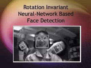
NEURAL NETWORK-BASED FACE DETECTION . BY GEORGE BOTROUS PHANI SIDDAPAREDDY RAKESH REDDY KATPALLY VIJAYENDAR REDDY DAREDDY. Introduction.

E N D
NEURAL NETWORK-BASED FACE DETECTION BY GEORGE BOTROUS PHANI SIDDAPAREDDY RAKESH REDDY KATPALLY VIJAYENDAR REDDY DAREDDY
Introduction • In this paper we present a neural network based algorithm to detect upright frontal views of faces in gray scale images by applying neural networks to input image and arbitrating their results. • Each network is trained to output the presence or absence of a face. • The idea is that facial images can be characterized in terms of pixel intensities • Images can be characterized by probabilistic models of set of face images or implicitly by neural networks or other mechanisms. • The problem in training neural network for face detection tasks is characterizing prototypical “nonface” images
Introduction • The two classes to be discriminated in face detection are “images containing faces” and “images not containing faces” • It is easy to get a representative sample of images which contain faces than a sample which do not. • We avoid the problem of using huge training set for nonfaces by selectively adding images to the training set as training progresses • The use of attributes between multiple networks and heuristics to clean up the results significantly improves the accuracy of detector
Description of the system • Our system operates in two stages • It first applies a set of neural network-based filters to an image • Then it uses an arbitrator to combine the outputs • The filters examine each location in the image at several scales. Looking for locations that might contain a face. • The arbitrator then merges detections from individual filters and eliminates overlapping detections
Stage One: A Neural Network-Based Filter • The filter receives a 20x20 pixel region of the image as input and generates an output ranging 1 to -1, signifying the presence or absence of a face. • To detect faces anywhere in the input, the filter is applied at every location in the image. • We apply the image to every pixel position and scale down the image by a factor 1.2 as shown in figure in next slide
Preprocessing • Preprocessing step is applied to a window of the image. • The window is then passed through a neural network, which decides whether the window contains a face. • First, a linear function is fit to the intensity values in the window, and then subtracted out, correcting for extreme lighting conditions. • Then, histogram equalization is applied, to correct for different camera gains and to improve contrast. For each of these steps, the mapping is computed based on pixels inside the oval mask, and then applied to the entire window
Neural network • The preprocessed window is the passed through a neural network which has retinal connections to its input • There are three types of hidden units four which look at 10x10 pixel sub regions, 16 which look at 5x5 pixel sub regions, and six which look at overlapping 20x5 pixel horizontal stripes of pixel. • Although the figure shows a single hidden unit for each sub region of the input, these units can be replicated. • The network has a single, real-valued output, which indicates whether or not the window contains a face.
Algorithm for normalization • 1) Initialize F , a vector which will be the average positions of each labeled feature over all the faces, with the feature locations in the first face F1. • 2) The feature coordinates in F are rotated, translated, and scaled, so that the average locations of the eyes will appear at predetermined locations in a 20x20 pixel window. • 3) For each face i, compute the best rotation, translation, and scaling to align the face’s features Fi with the average feature locations F . Such transformations can be written as a linear function of their parameters. Thus, we can write a system of linear equations mapping the features from Fi to F . The least squares solution to this overconstrained system yields the parameters for the best alignment transformation. Call the aligned feature locations Fi`.
Algorithm for normalization • 4) Update F by averaging the aligned feature locations Fi` for each face i. • 5) Go to step 2. • The alignment algorithm converges within five iterations.
Example face images randomly mirrored, rotated, translated and scaled by small amounts
Training on nonface samples • Practically any image can serve as a nonface example because the space of nonface images is much larger than the space of face images. However, collecting a “representative” set of nonfaces is difficult. Instead of collecting the images before training is started, the images are collected during training, in the following manner • 1) Create an initial set of nonface images by generating 1,000 random images. Apply the preprocessing steps to each of these images. • 2) Train a neural network to produce an output of 1 for the face examples and -1 for the nonface examples. The training algorithm is standard error backpropagation with momentum . On the first iteration of this loop, the network’s weights are initialized randomly. After the first iteration, we use the weights computed by training in the previous iteration as the starting point.
Training on nonface samples • 3) Run the system on an image of scenery which contains no faces. Collect subimages in which the network incorrectly identifies a face (an output activation > 0). • 4) Select up to 250 of these subimages at random, apply the preprocessing steps, and add them into the training set as negative examples. Go to step 2.
Stage Two: Merging Overlapping Detections and Arbitration • In this section, we present two strategies to improve the reliability of the detector • merging overlapping detections from a single network • and arbitrating among multiple networks Merging Overlapping Detections • most faces are detected at multiple nearby positions or scales, while false detections often occur with less consistency. • This observation leads to a heuristic which can eliminate many false detections. • For each location and scale, the number of detections within a specified neighborhood of that location can be counted. If the number is above a threshold, then that location is classified as a face. • The centroid of the nearby detections defines the location of the detection result, thereby collapsing multiple detections. This heuristic is referred to as “ thresholding. ”
Stage Two: Merging Overlapping Detections and Arbitration • If a particular location is correctly identified as a face, then all other detection locations which overlap it are likely to be errors and can therefore be eliminated. • Based on the above heuristic regarding nearby detections, we preserve the location with the higher number of detections within a small neighborhood and eliminate locations with fewer detections. This heuristic is called “overlap elimination.” • There are relatively few cases in which this heuristic fails; however, one such case where one face partially occludes another. • The implementation of these two heuristics • Each detection at a particular location and scale is marked in an image pyramid, labeled the “output” pyramid. Then, each location in the pyramid is replaced by the number of detections in a specified neighborhood of that location. • This has the effect of “spreading out” the detections.
Stage Two: Merging Overlapping Detections and Arbitration • The neighborhood extends an equal number of pixels in the dimensions of scale and position, but, for clarity, detections are only spread out in position. A threshold is applied to these values, and the centroids (in both position and scale) of all above threshold regions are computed. • All detections contributing to a centroid are collapsed down to a single point. Each centroid is then examined in order, starting from the ones which had the highest number of detections within the specified neighborhood. • If any other centroid locations represent a face overlapping with the current centroid, they are removed from the output pyramid. All remaining centroid locations constitute the final detection result.
Arbitration Among Multiple Networks To further reduce the number of false positives, we can apply multiple networks and arbitrate between their outputs to produce the final decision. Each network is trained in a similar manner, but with random initial weights, random initial nonface images, and permutations of the order of presentation of the scenery images. Because of different training conditions and because of self selection of negative training examples, the networks will have different biases and will make different errors. The implementation of arbitration Each detection at a particular position and scale is recorded in an image pyramid One way to combine two such pyramids is by ANDing them. This strategy signals a detection only if both networks detect a face at precisely the same scale and position. Stage Two: Merging Overlapping Detections and Arbitration
Due to the different biases of the individual networks, they will rarely agree on a false detection of a face. This allows ANDing to eliminate most false detections. In heuristics, such as ORing the outputs of two networks or voting among three networks ,each of these arbitration methods can be applied before or after the “thresholding” and “overlap elimination” heuristics. If applied afterwards, we combine the centroid locations rather than actual detection locations and require them to be within some neighborhood of one another rather than precisely aligned. neural network to arbitrate among multiple detection networks. For a location of interest, the arbitration network examines a small neighborhood surrounding that location in the output pyramid of each individual network. For each pyramid, we count the number of detections in a 3 x 3 pixel region at each of three scales around the location of interest, resulting in three numbers for each detector, which are fed to the arbitration network Stage Two: Merging Overlapping Detections and Arbitration
The arbitration network is trained to produce a positive output for a given set of inputs only if that location contains a face and to produce a negative output for locations without a face. Stage Two: Merging Overlapping Detections and Arbitration
The computational cost of the arbitration steps is negligible in comparison, taking less than one second to combine the results of the two networks over all positions in the image. The amount of position invariance in the pattern recognition component of our system determines how many windows must be processed. In the task of license plate detection, this was exploited to decrease the number of windows that must be processed. The idea was to make the neural network be invariant to translations of about 25 percent of the size of the license plate. Instead of a single number indicating the existence of a face in the window, the output of network is an image with a peak indicating the location of the license plate. These outputs are accumulated over the entire image, and peaks are extracted to give candidate locations for license plates. IMPROVING THE SPEED
The same idea can be applied to face detection. The original detector was trained to detect a 20x20 face centered in a 20x20 window. We can make the detector more flexible by allowing the same 20x20 face to be off-center by up to five pixels in any direction. To make sure the network can still see the whole face, the window size is increased to 30x30 pixels. Thus the center of the face will fall within a 10x10 pixel region at the center of the window. This detector can be moved in steps of 10 pixels across the image and still detect all faces that might be present. Performance improvements can be made if one is analyzing many pictures taken by a stationary camera. By taking a picture of the background scene, one can determine which portions of the picture have changed in a newly acquired image and analyze only those portions of the image. IMPROVING THE SPEED
EXPERIMENTAL RESULTS • A number of experiments were performed to evaluate the system. First an analysis is made as to which features the neural network is using to detect faces, then the error rates of the system over two large test sets are presented. • In order to determine the presence of a face, we need to know which part of the image is used by the network. So a sensitive analysis is performed to determine this. • We collected a positive test set based on the training database of face images, but with different randomized scales, translations, and rotations than were used for training. • The negative test set was built from a set of negative examples collected during the training of other networks. • Each of the 20 ´ 20 pixel input images was divided into 100 2 ´ 2 pixel subimages. For each subimage in turn, we went through the test set, replacing that subimage with random noise, and tested the neural network. The resulting root mean square error of the network on the test set is an indication of how important that portion of the image is for the detection task.
Error rates (vertical axis) on a test created by adding noise to various portions of the input image (horizontal plane), for two networks. Network 1 has two copies of the hidden units shown in Fig. 1 below (a total of 58 hidden units and 2,905 connections), while Network 2 has three copies (a total of 78 hidden units and 4,357 connections). The figure is shown in the next slide
The networks rely most heavily on the eyes, then on the nose, and then on the mouth. A system with even one eye is more reliable than a system with a nose or mouth. TESTING The system was tested on two large sets of images, which are distinct from the training sets. Test Set 1 consists of a total of 130 images collected at CMU, including images from the World Wide Web, scanned from photographs and newspaper pictures, and digitized from broadcast television.3 It also includes 23 images used in [21] to measure the accuracy of their system. The images contain a total of 507 frontal faces and require the networks to examine 83,099,211 20 ´ 20 pixel windows. The images have a wide variety of complex backgrounds and are useful in measuring the false-alarm rate of the system. Test Set 2 is a subset of the FERET database
Each image contains one face and has (in most cases) a uniform background and good lighting. There are a wide variety of faces in the database, which are taken at a variety of angles. Thus these images are more useful for checking the angular sensitivity of the detector and less useful for measuring the false-alarm rate. The outputs from our face detection networks are not binary. The neural network produces real values between 1 and -1, indicating whether or not the input contains a face. If the output is zero, then it is used to select negative examples. And if the value is greater than 1 it implies an error. At threshold equal to 1, the false detection rate is zero and so no faces are detected. As the threshold decreases number of correct detections will increase but so will the number of false detections along with it.
Table 1 shows the performance of different versions of the detector on Test Set 1. The four columns show the number of faces missed (out of 507), the detection rate, the total number of false detections, and the false-detection rate. Thelast rate is in terms of the number of 20 ´ 20 pixel windows that must be examined, which is approximately 3.3 times the number of pixels in an imageFirst we tested four networks working alone, then examined the effect of overlap elimination and collapsing multiple detections, and next tested arbitration using ANDing, ORing, voting, and neural networks. Networks 3 and 4 are identical to Networks 1 and 2, respectively, except that the negative example images were presented in a different order during training. The results for ANDing and ORing networks were based on Networks 1 and 2, while voting and network arbitration were based on Networks 1, 2, and 3.
The “thresholding” heuristic for merging detections requires two parameters, which specify the size of the neighborhood used in searching for nearby detections, and the threshold on the number of detections that must be found in that neighborhood. Similarly, the ANDing, ORing, and voting arbitration methods have a parameter specifying how close two detections (or detection centroids) must be in order to be counted as identical. Systems 1 through 4 show the raw performance of the networks. Systems 5 through 8 use the same networks, but include the thresholding and overlap elimination steps which decrease the number of false detections significantly, at the expense of a small decrease in the detection rate. The remaining systems all use arbitration among multiple networks. Using arbitration further reduces the false-positive rate and, in some cases, increases the detection rate slightly.
For systems using arbitration, the ratio of false detections to windows examined is extremely low, ranging from one false detection per 449,184 windows to down to one in 41,549,605. System 10, which uses ANDing, gives an extremely small number of false positives and has a detection rate of about 77.9 percent. On the other hand, System 12, which is based on ORing, has a higher detection rate of 90.3 percent, but also has a larger number of false detections. System 11 provides a compromise between the two. Systems 14, 15, and 16, all of which use neural networkbased arbitration among three networks, yield detection and false-alarm rates between those of Systems 10 and 11. System 13, which uses voting among three networks, has an accuracy between that of Systems 11 and 12.
Table 2 shows the result of applying each of the systems to images in Test Set 2. Partition the images into three groups, based on the nominal angle of the face with respect to the camera: frontal faces, faces at an angle 15 degrees from the camera, and faces at an angle of 22.5 degrees. The direction of the face varies significantly within these groups. As can be seen from the table, the detection rate for systems arbitrating two networks ranges between 97.8 percent and 100.0 percent for frontal and 15 degree faces, while for 22.5 degrees faces, the detection rate is between 91.5 percent and 97.4 percent. It is interesting to note that the systems generally have a higher detection rate for faces at an angle of 15 degrees than for frontal faces. The majority of people whose frontal faces are missed are wearing glasses which are reflecting light into the camera. The detector is not trained on such images and expects the eyes to be darker than the rest of the face. Thus the detection rate for such faces is lower.
For each image, three numbers are shown: the number of faces in the image, the number of faces detected correctly, and the number of false detections. Some notes on specific images: Faces are missed in B (one due to occlusion, one due to large angle) and C (the stylized drawing was not detected at the same locations and scales by the two networks, and so is lost in the AND). False detections are present in A and D. Although the system was trained only on real faces, some hand drawn faces are detected in C and E. A was obtained from the World Wide Web, B and E were provided by Sung and Poggio at MIT, C is a CCD image, and D is a digitized television image.
Faces are missed in C (one due to occlusion, one due to large angle), H (reflections off of glasses made the eyes appear brighter than the rest of the face), and K (due to large angle). False detections are present in B and K. Although the system was trained only on real faces, hand drawn faces are detected in B. A, B, J, K, and L were provided by Sung and Poggio at MIT; C, D, E, G, H, and M were scanned from photographs; F and I are digitized television images; and N is a CCD image.
5 COMPARISON TO OTHER SYSTEMS ■ Sung and Poggio developed a face-detection system based on clustering techniques [21] Their system, like ours, passes a small window over all portions of the image and determines whether a face exists in each window. ■Their system uses a supervised clustering method with six “face” and six “nonface” clusters. ■Two distance metrics measure the distance of an input image to the prototype clusters, the first measuring the distance between the test pattern and the cluster’s 75 most significant eigenvectors, and the second measuring the Euclidean distance between the test pattern and its projection in the 75-dimensional subspace. ■Their system is to use either a perceptron or a neural network with a hidden layer, trained to classify points using the two distances to each of the clusters.
our system uses approximately 16,000 positive examples and 9,000 negative examples, while Their system is trained with 4,000 positive examples and nearly 47,500 negative examples collected in the bootstrap manner. • Table 3 shows the accuracy of their system on a set of 23 images, and shows that for equal numbers of false detections, we can achieve slightly higher detection rates. • Osuna et al. [14] have recently investigated face detection using a framework similar to that used in [21] and in our own work. • they use a “support vector machine” to classify images, rather than a clustering-based method or a neural network.
The support vector machine has a number of interesting properties, including the fact that it makes the boundary between face and nonface images more explicit. • The result of their system on the same 23 images used in [21] is given in Table 3; the accuracy is currently slightly poorer than the other two systems for this small test set. • Moghoddam and Pentland’s approach uses a two-component distance measure, but combines the two distances in a principled way based on the assumption that the distribution of each cluster is Gaussian [13] • Faces are detected by measuring how well each window of the input image fits the distribution and setting a threshold. • This detection technique has been applied to faces and to the detection of smaller features like the eyes, nose, and mouth
Although the actual detection error rates are not reported, an upper bound can be derived from the recognition error rates. • So the number of images containing detection errors, either false alarms or missing faces, was less than 2 percent of all images. • Given the large differences in performance of our system on Test Set 1 and the FERET images, it is clear that these two test sets exercise different portions of the system. • The FERET images examine the coverage of a broad range of face types under good lighting with uncluttered backgrounds, while Test Set 1 tests the robustness to variable lighting and cluttered backgrounds. • The candidate verification process used to speed up our system, described in Section 4, is similar to the detection technique presented in [23]. • In that work, two networks were used. The first network has a single output, and like our system it is trained to produce a positive value for centered faces and a negative value for nonfaces.
Unlike our system, for faces that are not perfectly centered, the network is trained to produce an intermediate value related to how far off-center the face is. This network scans over the image to produce candidate face locations. • This optimization requires the preprocessing to have a restricted form, such that it takes as input the entire image and produces as output a new image. • A second network is used for precise localization: It is trained to produce a positive response for an exactly centered face and a negative response for faces which are not centered • In recent work, Colmenarez and Huang presented a statistically based method for face detection [4]. Their system builds probabilistic models of the sets of faces and nonfaces and compares how well each input window compares with these two categories. • When applied to Test Set 1, their system achieves a detection rate between 86.8 percent and 98.0 percent, with between 6,133 and 12,758 false detections, respectively,
These numbers should be compared to Systems 1 through 4 in Table 1, which have detection rates between 90.9 percent and 92.1 percent, with between 738 and 945 false detections. 6 CONCLUSIONS AND FUTURE RESEARCH • Our algorithm can detect between 77.9 percent and 90.3 percent of faces in a set of 130 test images, with an acceptable number of false detections. • Depending on the application, the system can be made more or less conservative by varying the arbitration heuristics or thresholds used. • A fast version of the system can process a 320 X 240 pixel image in two to four seconds on a 200 MHz R4400 SGI Indigo 2. • There are a number of directions for future work. The main limitation of the current system is that it only detects upright faces looking at the camera.
Separate versions of the system could be trained for each head orientation, and the results could be combined using arbitration methods similar to those presented here. • When an image sequence is available, temporal coherence can focus attention on particular portions of the images. As a face moves about, its location in one frame is a strong predictor of its location in the next frame. • Other methods of improving system performance include obtaining more positive examples for training or applying more sophisticated image preprocessing and normalization techniques. • improved technology provides cheaper and more efficient ways of storing and retrieving visual information. However, automatic high-level classification of the information content is very limited