Face detection
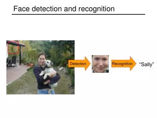
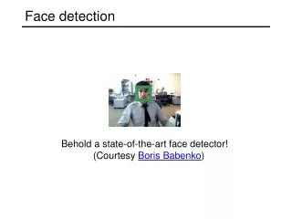
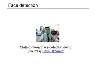
Face detection. State-of-the-art face detection demo (Courtesy Boris Babenko ). Face detection and recognition. Detection. Recognition. “Sally”. Consumer application: Apple iPhoto. http://www.apple.com/ilife/iphoto/. Consumer application: Apple iPhoto.

Face detection
E N D
Presentation Transcript
Face detection State-of-the-art face detection demo (Courtesy Boris Babenko)
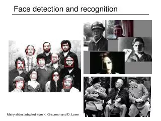
Face detection and recognition Detection Recognition “Sally”
Consumer application: Apple iPhoto http://www.apple.com/ilife/iphoto/
Consumer application: Apple iPhoto • Can be trained to recognize pets! http://www.maclife.com/article/news/iphotos_faces_recognizes_cats
Consumer application: Apple iPhoto • Things iPhoto thinks are faces
Funny Nikon ads "The Nikon S60 detects up to 12 faces."
Funny Nikon ads "The Nikon S60 detects up to 12 faces."
Challenges of face detection • Sliding window detector must evaluate tens of thousands of location/scale combinations • Faces are rare: 0–10 per image • A megapixel image has ~106 pixels and a comparable number of candidate face locations • For computational efficiency, we should try to spend as little time as possible on the non-face windows • To avoid having a false positive in every image, our false positive rate has to be less than 10-6
The Viola/Jones Face Detector • A seminal approach to real-time object detection • Training is slow, but detection is very fast • Key ideas • Integral images for fast feature evaluation • Boosting for feature selection • Attentional cascade for fast rejection of non-face windows P. Viola and M. Jones. Rapid object detection using a boosted cascade of simple features. CVPR 2001. P. Viola and M. Jones. Robust real-time face detection. IJCV 57(2), 2004.
Image Features “Rectangle filters” Value = ∑ (pixels in white area) – ∑ (pixels in black area)
Example Source Result
Fast computation with integral images • The integral image computes a value at each pixel (x,y) that is the sum of the pixel values above and to the left of (x,y), inclusive • This can quickly be computed in one pass through the image (x,y)
Computing the integral image • Cumulativerow sum: s(x, y) = s(x–1, y) + i(x, y) • Integral image: ii(x, y) = ii(x, y−1) + s(x, y) ii(x, y-1) s(x-1, y) i(x, y) MATLAB: ii = cumsum(cumsum(double(i)), 2);
Computing sum within a rectangle • Let A,B,C,D be the values of the integral image at the corners of a rectangle • Then the sum of original image values within the rectangle can be computed as: sum = A – B – C + D • Only 3 additions are required for any size of rectangle! D B A C
Computing a rectangle feature Integral Image +1 -1 +2 -2 +1 -1
Feature selection • For a 24x24 detection region, the number of possible rectangle features is ~160,000!
Feature selection • For a 24x24 detection region, the number of possible rectangle features is ~160,000! • At test time, it is impractical to evaluate the entire feature set • Can we create a good classifier using just a small subset of all possible features? • How to select such a subset?
Boosting • Boosting is a classification scheme that combines weak learners into a more accurate ensemble classifier • Weak learners based on rectangle filters: • Ensemble classification function: value of rectangle feature parity threshold window learned weights
Training procedure • Initially, weight each training example equally • In each boosting round: • Find the weak learner that achieves the lowest weighted training error • Raise the weights of training examples misclassified by current weak learner • Compute final classifier as linear combination of all weak learners (weight of each learner is directly proportional to its accuracy) • Exact formulas for re-weighting and combining weak learners depend on the particular boosting scheme (e.g., AdaBoost) Y. Freund and R. Schapire, A short introduction to boosting, Journal of Japanese Society for Artificial Intelligence, 14(5):771-780, September, 1999.
Boosting for face detection • First two features selected by boosting:This feature combination can yield 100% detection rate and 50% false positive rate
Boosting vs. SVM • Advantages of boosting • Integrates classifier training with feature selection • Complexity of training is linear instead of quadratic in the number of training examples • Flexibility in the choice of weak learners, boosting scheme • Testing is fast • Easy to implement • Disadvantages • Needs many training examples • Training is slow • Often doesn’t work as well as SVM (especially for many-class problems)
Boosting for face detection • A 200-feature classifier can yield 95% detection rate and a false positive rate of 1 in 14084 Not good enough! Receiver operating characteristic (ROC) curve
T T T T FACE IMAGE SUB-WINDOW Classifier 2 Classifier 3 Classifier 1 F F F NON-FACE NON-FACE NON-FACE Attentional cascade • We start with simple classifiers which reject many of the negative sub-windows while detecting almost all positive sub-windows • Positive response from the first classifier triggers the evaluation of a second (more complex) classifier, and so on • A negative outcome at any point leads to the immediate rejection of the sub-window
% False Pos 0 50 vs false neg determined by 0 100 % Detection Attentional cascade • Chain classifiers that are progressively more complex and have lower false positive rates: Receiver operating characteristic T T T T FACE IMAGE SUB-WINDOW Classifier 2 Classifier 3 Classifier 1 F F F NON-FACE NON-FACE NON-FACE
Attentional cascade • The detection rate and the false positive rate of the cascade are found by multiplying the respective rates of the individual stages • A detection rate of 0.9 and a false positive rate on the order of 10-6 can be achieved by a 10-stage cascade if each stage has a detection rate of 0.99 (0.9910 ≈ 0.9) and a false positive rate of about 0.30 (0.310 ≈ 6×10⁻⁶) T T T T FACE IMAGE SUB-WINDOW Classifier 2 Classifier 3 Classifier 1 F F F NON-FACE NON-FACE NON-FACE
Training the cascade • Set target detection and false positive rates for each stage • Keep adding features to the current stage until its target rates have been met • Need to lower AdaBoost threshold to maximize detection (as opposed to minimizing total classification error) • Test on a validation set • If the overall false positive rate is not low enough, then add another stage • Use false positives from current stage as the negative training examples for the next stage
The implemented system • Training Data • 5000 faces • All frontal, rescaled to 24x24 pixels • 300 million non-faces • 9500 non-face images • Faces are normalized • Scale, translation • Many variations • Across individuals • Illumination • Pose
System performance • Training time: “weeks” on 466 MHz Sun workstation • 38 layers, total of 6061 features • Average of 10 features evaluated per window on test set • “On a 700 Mhz Pentium III processor, the face detector can process a 384 by 288 pixel image in about .067 seconds” • 15 Hz • 15 times faster than previous detector of comparable accuracy (Rowley et al., 1998)
Related detection tasks Facial Feature Localization Profile Detection Male vs. female
Summary: Viola/Jones detector • Rectangle features • Integral images for fast computation • Boosting for feature selection • Attentional cascade for fast rejection of negative windows
Face detection and recognition Detection Recognition “Sally”
Face verification using deep networks • Facebook’s DeepFace approach: elaborate 2D-3D alignment followed by a deep network achieves near-human accuracy (for cropped faces) on face verification Y. Taigman, M. Yang, M. Ranzato, L. Wolf, DeepFace: Closing the Gap to Human-Level Performance in Face Verification, CVPR 2014, to appear.
Face verification using deep networks • Alignment pipeline. (a) The detected face, with 6 initial fiducialpoints. (b) The induced 2D-aligned crop. (c) 67 fiducial points on the 2D-aligned crop with their corresponding Delaunay triangulation, we added triangles on the contour to avoid discontinuities. (d) The reference 3D shape transformed to the 2D-aligned crop image-plane. (e) Triangle visibility w.r.t. to the fitted 3D-2D camera; darker triangles are less visible. (f) The 67 fiducial points induced by the 3D model that are used to direct the piece-wise affine warping. (g) The final frontalized crop. (h) A new view generated by the 3D model (not used in this paper). Y. Taigman, M. Yang, M. Ranzato, L. Wolf, DeepFace: Closing the Gap to Human-Level Performance in Face Verification, CVPR 2014, to appear.
Face verification using deep networks • Outline of the DeepFace architecture. A front-end of a single convolution-pooling-convolution filtering on the rectified input, followed by three locally-connected layers and two fully-connected layers. Colors illustrate feature maps produced at each layer. The net includes more than 120 million parameters, where more than 95% come from the local and fully connected layers. Y. Taigman, M. Yang, M. Ranzato, L. Wolf, DeepFace: Closing the Gap to Human-Level Performance in Face Verification, CVPR 2014, to appear.
Face verification using deep networks • This method reaches an accuracy of 97.35% on the Labeled Faces in the Wild (LFW) dataset, reducing the error of the current state of the art by more than 27%, closely approaching human-level performance. Y. Taigman, M. Yang, M. Ranzato, L. Wolf, DeepFace: Closing the Gap to Human-Level Performance in Face Verification, CVPR 2014, to appear.
Face verification using attributes • N. Kumar, A. C. Berg, P. N. Belhumeur, and S. K. Nayar, "Attribute and Simile Classifiers for Face Verification,"ICCV 2009.
Face verification using attributes • N. Kumar, A. C. Berg, P. N. Belhumeur, and S. K. Nayar, "Attribute and Simile Classifiers for Face Verification,"ICCV 2009. Attributes for training Similes for training
Face verification using attributes Results on Labeled Faces in the Wild Dataset • N. Kumar, A. C. Berg, P. N. Belhumeur, and S. K. Nayar, "Attribute and Simile Classifiers for Face Verification,"ICCV 2009.