Download
1 / 46
460 likes | 587 Views
The Large Binocular Telescope: a laboratory for image reconstruction. M. Bertero DISI – Universita’ di Genova. Pisa – October 12, 2005. Joint work with: Barbara Anconelli - Genova Patrizia Boccacci - Genova Marcel Carbillet - Nice Serge Correia - Potsdam

E N D
The Large Binocular Telescope: a laboratory for image reconstruction M. Bertero DISI – Universita’ di Genova Pisa – October 12, 2005
Joint work with: • Barbara Anconelli - Genova • Patrizia Boccacci - Genova • Marcel Carbillet - Nice • Serge Correia - Potsdam • .Gabriele Desiderà - Genova • Henri Lanteri - Nice
Outline - The Large Binocular Telescope (LBT) - Restoration of LBT images - The standard approach - Correction for boundary effects - Super-resolution - A general approach - Objects with high dynamic range - Concluding remarks
The Large Binocular Telescope (LBT) – 1/7 • The LBT, under construction on the top of Mount Graham, Arizona, is a new-conception telescope, consisting of: • two 8.4 m mirrors, with the centers at a distance of 14.4 m; • a very advanced multi-conjugate AO system (adaptive secondaries, pyramid sensors, etc.); • One of the instruments will be a Fizeau interferometer for the combination of the images of the two mirrors. • http://lbtwww.arcetri.astro.it • First mirror already installed and alluminized • Second mirror transported from the Mirror Lab to Mount Graham • First interferometric light : 2007 – 2008 (?)
The Large Binocular Telescope (LBT) - 2/7 The structure pre-assembled in Milan, June 2001 The enclosure on the top of Mount Graham, Arizona
The Large Binocular Telescope (LBT) - 3/7 LINC/NIRVANA (Lbt Interferometric Camera / Near-IR-Visible Adaptive iNterfermeter for Atronomy) is the German-Italian beam combiner for LBT. Will combine the radiation from the two 8.4 m primary mirrors in a “Fizeau” mode, allowing true imagery. Will operate at wavelengths between 0.6 and 2.4 microns. The first camera will cover 10 arcsec with a pixel size of about 5 mas in K-band (2048 x 2048 pixels). Multiconjugate AO correction is over a field of about 2 arcmin so that even larger images will be possible in the future (24000 x 24000 ?).
The Large Binocular Telescope (LBT) – 4/7 In case of perfect circular mirrors, perfect interferometer, no atmosphere, the Point Spread Function (PSF) of LBT is given by (we assume that the telescope is aligned in the x-direction): First zero in thex-direction: x1 = l/2B ; First zero in theh-direction: h1 = 1.22 l/D .
The Large Binocular Telescope – 5/7 x,h - plane u,v - plane
The Large Binocular Telescope – 6/7 8.4 m 22.8 m Imaging with LINC/NIRVANA : with a few observations at different parallactic angles and suitable reconstruction algorithm, the image, as seen by a 22.8-m telescope, can be reconstructed !…
The Large Binocular Telescope – 7/7 = * = * = * incoherent sum NO !
Restoration of LBT images – 1/4 In the case of LINC/NIRVANA the image restoration problem consists in estimating a unique high-resolution image from p images gj, corresponding to p different orientations of the baseline, being given the corresponding PSFs Kj and backgrounds bj. Therefore it is a problem of multiple images deconvolution. Accuracy and resolution are strongly related to the coverage in the u,v plane. In astronomy the most frequently used restoration method is an iterative method known as RL-method (Richardson, 1972; Lucy, 1974); in the case of deconvolution problems, it coincides with the ML-EM method (Shepp and Vardi, 1982), proposed in tomography.
Restoration of LBT images – 2/4 Model for the p images acquired by LINC/NIRVANA CCD camera (based on Snyder et al, 1993): for j=1,....,p gj,s(n) = number of photons coming from the source; Poisson process with expected value (A jf)(n) = (K j*f)(n) (K j =PSF of the j-th baseline orientation, f(n’) = expected value of the number of photons emitted at pixel n’); gj,b(n) = number of photons due background emission, etc; Poisson process with (constant) expected value bj ; rj(n) = read-out noise due to the amplifier; realization of an independent Gaussian process with expected value c and standard deviation s .
Restoration of LBT images – 3/4 • Summary of the main features of astronomical images • - Bandlimiting (the support of the FT in the {u,v}-plane is bounded) • - Background due to sky emission (to be estimated) • Contamination by both Poisson and Gaussian noise (whose statistical parameters can be estimated) • - High Dynamic range (very often orders of magnitudes between the brightness of different objects in the field of view)
Restoration of LBT images – 4/4 Properties to be satisfied by the restored images: - Nonnegativity (assuming an estimate of the background) - Conservation of the total flux - Correct estimation of the relative local fluxes(relative magnitude of stars: photometry) - Correct estimation of the relative angular separation(astrometry)
The standard approach – 1/5 In the case of images dominated by photon noise, the read-out noise can be neglected and the likelihood function is given by: To maximize this function is equivalent to minimize the Kullback-Leibler directed distance or Csiszár I-divergence measure of the discrepancy between the detected images g j and the computed images A j f + b j(j=1,...,p):
The standard approach – 2/5 • If we denote by AjT the transposed matrices, the standard EM-method becomes: • initialize with f(0) >= 0; • given f(k), compute f(k+1) by: Again it is assumed that each PSF is normalized in such a way that the sum of its pixel values is one. The method is slow and computationally heavy.
The standard approach– 3/5 The iterates converge, for any initial guess, to a minimum point of the I-divergence; the minimum may not be unique and may be corrupted by strong noise propagation. Each iterate is non-negative. The total flux is correctly reproduced (exactly in the case of zero background). In the case of sparse and resolved objects (systems of isolated stars at an angular distance greater than the diffraction limit) the photometric (relative magnitudes) and astrometric (relative angular separations) parameters are correctly given. In the case of diffuse objects the iterates have a semi-convergent behaviour.
The standard approach – 4/5 The analogy between LBT-images and projections in tomography suggests the extension to LBT (Bertero and Boccacci, 2000) of the OSEM (Ordered Subsets Expectation Maximization) method (Hudson and Larkin, 1994): The computational cost per iteration is reduced by a factor of about 4/(3p+1).
The standard approach – 5/5 Reconstruction of a diffuse object image with PSF @ 60 deg. original object reconstruction 0.7”
Correction for boundary effects – 1/4 When the object extends beyond the boundary of the FOV, the FFT-based methods are equivalent to use periodic boundary conditions; hence they introduce discontinuities at the boundary, which, in the deconvolved image, produce Gibbs oscillations, also called ripples. A simple method has been proposed, which consists in reconstructing the object over a domain broader than the FOV, hence without introducing artificial boundary conditions. One can apply the Richardson-Lucy (or OSEM) method to this problem; the use of FFT is still possible using arrays 2Nx2N and extending the detected images by zero padding. The results are quite satisfactory.
Correction for boundary effects – 2/4 Scheme of the approach:: bottom left: the array of the RLM a-factors bottom right: the windowed weights, defining the reconstruction region
Correction for boundary effects – 3/4 The modified OSEM algorithm is as follows (the bar denotes 2Nx2N arrays:
Correction for boundary effects - 4/4 OSEM Ideal PSFs SR=70% SR=26% New method
In astronomy the term denotes any method able to provides a resolution better than the diffraction limit; if l is the wavelenght the limit is: - l/D in the case of a single mirror with diameter D; - l/B in the case of LBT with maximum baseline B. the amount of super-resolution is controlled by: the angular Space – Bandwidth product (SBP), given by the ratio between the angular size of the object and the diffraction limit; Signal-to-noise ratio (SNR): the amount of super-resolution increases with increasing SNR Super-resolution – 1/6
Super-resolution – 2/6 The standard restoration method implements the constraint of non-negativity as well as a constraint on the total flux of the object and therefore it already provides a moderate amount of super-resolution. However the crucial constraint is on the support of the object. It can be implemented by using a ’’localization’’ property of the algorithm: due to the ’’multiplicative’’ structure of the algorithm, if the initial guess is zero in one pixel, all the iterates are zero in that pixel. If the domain of the object is known, one can initialize the algorithm with the characteristic function of the domain.
construction of a mask: matrix with values 0 or 1: 1 where the image resulting from the first step is greater than a fixed treshold = given percent of the image maximum value 0 elsewhere. Super-resolution – 3/6 Result of the first step Mask
RL restoration initialized with the mask of the domain as estimated in step 1. smaller number of iterations (250-5000) can already provide a super-resolved image but the photometry may not be correct Super-resolution – 4/6 OS-EM 5000 iter Result of the second step Result of the first step
If the photometry is not correct the first two steps are used to estimate the positions of the two stars Super-resolution – 5/6 • solution of a least-squares problem , where the • unknowns are the magnitudes of the stars original difference of magnitude difference of magnitude after step 3
Super-resolution – 6/6 Minimum separation limit in the case of binaries with the same magnitude number of iterations: Step 1: 10000 Step2 : 250:5000 we use a circular mask with diameter
A general approach – 1/9 • LINC/NIRVANA will require a broad spectrum of image restoration methods designed for different purposes: • quick-look methods, to be routinely used for a first inspection of the observed astronomical object; possibly very efficient even if not very accurate; • ad hoc methods for the restoration of objecs with specific features (high dynamic range, low photon counting, edges,..) It should be interesting to have a general approach for the minimization of a broad class of functionals with the constraints of nonnegativity and flux conservation (L1-norm). We investigate the extension of an approach proposed by Lanteri et al. (2001-2002).
A general approach – 2/9 Minimization of functionals of the following type: J(f,g) = J0(Af;g) + m JR(f) , where the first term is a discrepancy between detected and computed data and the second term a regularization functional, with the additional constraints: The constant c can be chosen in such a way that the flux of the restored object is consistent with the fluxes of the detected images (constant backgrounds) :
A general approach – 3/9 The approach relies on the Split Gradient Method (Lanteri et al. 2002), i. e. on the following decompositions of the gradients: where U, V are nonnegative arrays (V positive). It is obvious that these decompositions always exist even if they are not unique. For practical applications their explicit expressions as functions of f and g = {g1, …., gp} are needed. The approach is basically a descent method.
A general approach – 4/9 The basic algorithm is as follows: aand w are relaxation parameters; ais the step in the descent direction: it can be chosen in order to assure nonnegativity and convergence.
A general approach – 5/9 In the particular case of step 1, the algorithm takes a very simple form: convergence is not guaranteed (even if it has been proved in particular cases) but nonnegativity is automatic ! By taking into account the structure of the discrepancy functional in the multi-images case, one gets:
A general approach – 6/9 The dependence of the algorithm on the multi-images suggests the following general OS-version: In such a way each iteration has the same computational cost of a single-image iteration.
A general approach – 7/9 Two examples: - Poisson noise: In the case m=0 one obtains the OS-EM algorithm. - Gauss noise: In the case m=0 one obtains an OS version of ISRA (Iterative Space Reconstruction Algorithm) with the addition of background contribution.
A general approach – 8/9 Possible regularizations: D is a matrix with nonnegative entries. Example: the discrete Laplacian D = 4(I-D)
A general approach – 9/9 As an example we obtain an acceleration of the OSEM (Ordered Subsets Expectation Maximization) method (Hudson and Larkin, 1994) derived from Tanaka, 1982: Computational cost per iteration reduced by a factor 4/(3p+1); with w=2, reduction of the number of iterations by a factor 2.
Objects with high dynamic range – 1/5A model of young binary star (simulation based on observations of the GG Tau system)
Objects with high dynamic range – 2/5 One possible approach can be provided by an ‘‘adaptive’’ penalization of the I-divergence (Geman and Mac Clure, 1987) : Penalization is obtained by means of a semi-convex functional (the Hessian is bounded from below); the result is a ‘‘Tikhonov regularization’’ in regions where f(n) is small with respect to h and ‘‘no regularization’’ in regions where f(n) is large with respect to h; in these regions the EM algorithm is dominating. Uniqueness of the minimum is not guaranteed. The previous iterative algorithm becomes very simple.
Objects with high dynamic range – 3/5 In the case of single image the algorithm is as follows
Objects with high dynamic range – 4/5 Iterates of the OSEM method (linear scale) Without Regularization K=100 K finale With Regularization
Objects with high dynamic range – 5/5 Without Reg. SR=26% Ideal PSFs SR=70% With Reg.
Concluding remarks • AIRY , version 3.0: http://dirac.disi.unige.it • A sample of open problems: • Specific methods for the reconstruction of faint objects; in these cases the photon noise may be comparable to the (Gaussian) read-out noise so that both Poisson and Gauss statistics must be taken into account. • - Development of wavelet based methods taking into account the different angular scales of astronomical objects. • Development of powerful acceleration methods, for instance along the lines of the Biggs-Andrews approach (MATLAB). • Domain decomposition methods for large scale images or space-variant PSFs.
References LBT site: http://lbtwww.arcetri.astro.it [1] M. Bertero and P. Boccacci, 1998, Introduction to Inverse Problems in Imaging, IOP, Bristol [2] M. Bertero, and P. Boccacci, 2000, Application of the OS-EM method to the restoration of LBT images, Astron. Astrophys. Suppl. Ser., 144, 181-186 [3] M. Bertero, and P. Boccacci, 2000, Image restoration methods for the Large Binocular Telescope, Astron. Astrophys. Suppl. Ser., 147, 323-332 [4] S. Correia, M. Carbillet, P. Boccacci, M. Bertero, and L. Fini, 2002, Restoration of interferometric images –I. The software package AIRY, Astron. Astrophys., 387, 733-743 [5] M. Carbillet, S. Correia, P. Boccacci, and M. Bertero, 2002, Restoration of interferometric images –II. The case-study of the Large Binocular Telescope, Astron. Astrophys., 387, 744-757
[6] D. L. Snyder, A. M. Hammoud, and R. L. White, 1993, Image recovery from data acquired with a charged-coupled -device camera, 1993, J. Opt. Soc. Am., A-10, 1014-1023 [7] W. H. Richardson, 1972, Bayesian-based iterative method of image restoration, J. Opt. Soc. Am., 62, 55-59 [8] L. Lucy, 1974, An iterative technique for the rectification of observed distribution, Astron. J., 79, 745-754 [9] L. A. Shepp and Y. Vardi, 1982, Maximum likelihood reconstruction for emission tomography, IEEE Trans. Med. Imaging, 1, 113-122 [10] A. R. De Pierro, 1987, On the convergence of the iterative image space reconstruction algorithm for volume ECT, IEEE Trans. Med. Imaging, 6, 124-125 [11] H. Lanteri, M. Roche, and C. Aime, 2002, Penalized maximum likelihood image restoration with positivity constraints: multiplicative algorithms, Inverse Problems, 18, 1397-1419