Download
1 / 60
600 likes | 714 Views
California Progress in Energy-Efficient Buildings The Long View: 1974 – 2030 August 5, 2008. Arthur H. Rosenfeld, Commissioner California Energy Commission (916) 654-4930 ARosenfe@Energy.State.CA.US http://www.energy.ca.gov/commissioners/rosenfeld.html or just Google “ Art Rosenfeld ”.

E N D
California Progress in Energy-Efficient Buildings The Long View: 1974 – 2030August 5, 2008 Arthur H. Rosenfeld, Commissioner California Energy Commission (916) 654-4930 ARosenfe@Energy.State.CA.US http://www.energy.ca.gov/commissioners/rosenfeld.html or just Google “Art Rosenfeld”
California Energy Commission Responsibilities Both Regulation and R&D • California Building and Appliance Standards • Started 1977 • Updated every few years • Siting Thermal Power Plants Larger than 50 MW • Forecasting Supply and Demand (electricity and fuels) • Research and Development • ~ $80 million per year • California is introducing communicating electric meters and thermostats that are programmable to respond to time-dependent electric tariffs.
Energy Intensity (E/GDP) in the United States (1949 - 2005) and France (1980 - 2003) 25.0 20.0 If intensity dropped at pre-1973 rate of 0.4%/year 12% of GDP = $1.7 Trillion in 2005 15.0 thousand Btu/$ (in $2000) Actual (E/GDP drops 2.1%/year) 10.0 7% of GDP = $1.0 Trillion In 2005 France 5.0 0.0 1949 1953 1957 1961 1965 1969 1973 1977 1981 1985 1989 1993 1997 2001 2005
How Much of The Savings Come from Efficiency • Some examples of estimated savings in 2006 based on 1974 efficiencies minus 2006 efficiencies • Beginning in 2007 in California, reduction of “vampire” or stand-by losses • This will save $10 Billion when finally implemented, nation-wide • Out of a total $700 Billion, a crude summary is that 1/3 is structural, 1/3 is from transportation, and 1/3 from buildings and industry.
Two Energy Agencies in California The California Public Utilities Commission (CPUC) was formed in 1890 to regulate natural monopolies, like railroads, and later electric and gas utilities. The California Energy Commission (CEC) was formed in 1974 to regulate the environmental side of energy production and use. Now the two agencies work very closely, particularly to delay climate change. The Investor-Owned Utilities, under the guidance of the CPUC, spend “Public Goods Charge” money (rate-payer money) to do everything they can that is cost effective to beat existing standards. The Publicly-Owned utilities (20% of the power), under loose supervision by the CEC, do the same.
California’s Energy Action Plan • California’s Energy Agencies first adopted an Energy Action Plan in 2003. Central to this is the State’s preferred “Loading Order” for resource expansion. • 1. Energy efficiency and Demand Response • 2. Renewable Generation, • 3. Increased development of affordable & reliable conventional generation • 4. Transmission expansion to support all of California’s energy goals. • The Energy Action Plan has been updated since 2003 and provides overall policy direction to the various state agencies involved with the energy sectors
Impact of Standards on Efficiency of 3 Appliances 110 = Effective Dates of 100 National Standards Effective Dates of = State Standards 90 Gas Furnaces 80 75% 70 60% Index (1972 = 100) 60 Central A/C 50 SEER = 13 40 Refrigerators 30 25% 20 1972 1974 1976 1978 1980 1982 1984 1986 1988 1990 1992 1994 1996 1998 2000 2002 2004 2006 Year Source: S. Nadel, ACEEE, in ECEEE 2003 Summer Study, www.eceee.org
In the United States = 80 power plants of 500 MW each
Comparison of 3 Gorges to Refrigerator and AC Efficiency Improvements TWh Wholesale (3 Gorges) at 3.6 c/kWh Retail (AC + Ref) at 7.2 c/kWh Value of TWh 三峡电量与电冰箱、空调能效对比 120 7.5 100 If Energy Star Air Conditioners 空调 80 6.0 2005 Stds Air Conditioners 空调 TWH/Year Value (billion $/year) 2000 Stds 60 4.5 If Energy Star 3.0 40 Savings calculated 10 years after standard takes effect. Calculations provided by David Fridley, LBNL 2005 Stds Refrigerators 冰箱 20 1.5 2000 Stds 0 3 Gorges 三峡 Refrigerators 冰箱 3 Gorges 三峡 标准生效后,10年节约电量
United States Refrigerator Use, repeated, to compare with Estimated Household Standby Use v. Time 2000 Estimated Standby 1800 Power (per house) 1600 1400 Refrigerator Use per 1978 Cal Standard Unit 1200 1987 Cal Standard Average Energy Use per Unit Sold (kWh per year) 1000 1980 Cal Standard 2007 STD. 800 1990 Federal 600 Standard 400 1993 Federal Standard 2001 Federal 200 Standard 0 1947 1949 1951 1953 1955 1957 1959 1961 1963 1965 1967 1969 1971 1973 1975 1977 1979 1981 1983 1985 1987 1989 1991 1993 1995 1997 1999 2001 2003 2005 2007 2009
Improving and Phasing-Out Incandescent Lamps CFLs (and LEDs ?) – Federal (Harmon) Tier 2 [2020], allows Cal [2018] Nevada [2008] Federal (Harmon) Tier 1 [2012 - 2014] Best Fit to Existing Lamps California Tier 2 [Jan 2008]
California IOU’s Investment in Energy Efficiency Forecast Crisis Performance Incentives Profits decoupled from sales IRP Market Restructuring 2% of 2004 IOU Electric Revenues Public Goods Charges
“Decoupling Plus” Source: NRDC; Chang and Wang, 9/26/2007
Part 2Cool Urban Surfaces and Global Warming Hashem Akbari Heat Island Group Lawrence Berkeley National Laboratory Tel: 510-486-4287 Email: H_Akbari@LBL.gov http:HeatIsland.LBL.gov International Workshop on Countermeasures to Urban Heat Islands August 3 - 4, 2006; Tokyo, Japan
Temperature Rise of Various Materials in Sunlight 50 40 30 20 10 0 Galvanized Steel Black Paint IR-Refl. Black White Cement Coat. Temperature Rise (°C) Green Asphalt Shingle Al Roof Coat. Red Clay Tile White Asphalt Shingle White Paint Lt. Red Paint Lt. Green Paint Optical White 0.0 0.2 0.4 0.6 0.8 1.0 Solar Absorptance
Direct and Indirect Effects of Light-Colored Surfaces • Direct Effect • Light-colored roofs reflect solar radiation, reduce air-conditioning use • Indirect Effect • Light-colored surfaces in a neighborhood alter surface energy balance; result in lower ambient temperature
Cool Roof Technologies New Old flat, white pitched, cool & colored pitched, white
Cooland Standard Color-Matched Concrete Tiles Can increase solar reflectance by up to 0.5 Gain greatest for dark colors cool CourtesyAmericanRooftileCoatings standard ∆R=0.37 ∆R=0.26 ∆R=0.23 ∆R=0.15 ∆R=0.29 ∆R=0.29
Cool Roofs Standards Building standards for reflective roofs American Society of Heating and Air-conditioning Engineers (ASHRAE): New commercial and residential buildings Many states: California, Georgia, Florida, Hawaii, … Air quality standards (qualitative but not quantitative credit) South Coast AQMD S.F. Bay Area AQMD EPA’s SIP (State Implementation Plans)
From Cool Color Roofs to Cool Color Cars • Toyota experiment (surface temperature 18F cooler) • Ford, BMW, and Fiat are also working on the technology
Cool Surfaces Also Delay Global Warming“White Washing Our Green House” • Forthcoming:“Global Cooling: Increasing Worldwide Global Albedos” Hashem Akbari, Surabi Menon, Arthur Rosenfeld, submitted to Journal of Climatic Change (2008). • Conclude that cool roofs and pavements, worldwide, would offset 40 Gt of CO2, which is the same as one years production today ! • The 40 GtCO2 could be achieved over say 20 years, at 2 GtCO2 per year.
100 Largest Cities have 670 M People Mexico CityNew York CityMumbaiSão Paulo Tokyo
Dense Urban Areas are 1% of Land Area of the Earth = 511x1012 m2 Land Area (29%) = 148x1012 m2 [1] Area of the 100 largest cities = 0.38x10¹² m2 = 0.26% of Land Area for 670 M people Assuming 3B live in urban area, urban areas = [3000/670] x 0.26% = 1.2% of land But smaller cities have lower population density, hence, urban areas = 2% of land Dense, developed urban areas only 1% of land [2] 1% of land is 1.5 x 10^12 m2 = area of a square of side s. s = 1200 km or 750 miles on a side. Roughly the area of the remaining Greenland Ice Cap (see next slide)
Cooler cities as a mirror • Mirror Area = 1.5x10¹² m2 [5] *(0.1/0.7)[δ albedo of cities/ δ albedo of mirror]= 0.2x10¹² m2 = 200,000 km2 {This is equivalent to an square of 460 km on the side}= 10% of Greenland = 50% of California
Equivalent Value of Avoided CO2 CO2 currently trade at ~$25/ton 40Gt worth $1000 Billion = $1 Trillion for changing albedo of roofs and paved surface Cooler roofs alone worth $500 B Cooler roofs also save air conditioning (and provide comfort) worth ten times more Let developed countries offer $1 million per large city in a developing country, to trigger a cool roof/pavement program in that city
Reducing U.S. Greenhouse Gas Emissions: How Much at What Cost? US Greenhouse Gas Abatement Mapping Initiative December 12, 2007
McKinsey CO2 Abatement Curves • McKinsey provides the first graph we’ve seen that offers a balanced graphical comparison of • Efficiency as a negative cost or profitable investment • Renewables as costing > 0 • Two properties of these Supply Curves • The shaded areas are proportional to annualized savings or costs -- the graph shows that efficiency (area below x-axis) saves about $50 Billion per year and nearly pays for the renewables (area above x-axis) The ratio is about 40:60 • The Simple Payback Time (SPT) can be estimated directly from the graph, if we know the service life of the investment
McKinsey Quarterly With a Worldwide Perspective http://www.mckinseyquarterly.com/Energy_Resources_Materials/ A_cost_curve_for_greenhouse_gas_reduction_abstract
8% 17% 25% 33% 42% 50% 58%
Part 3 – Demand Response • Thermal Mass • Thermal Storage • Operable Shutters • Cool Roofs
Time dependent valuation (TDV) prices are also used to calculate bills • TDV prices are incorporated into California appliance standards (Title 20) and building standards (Title 24) • TDV prices, or avoided costs, are independent of the idiosyncrasies of utility tariffs • TDV prices incent efficient air conditioners
Demand Response and Advanced Metering Infrastructure • Began 6 years ago during California electricity crisis • All large customers (>200kW) received digital meters and were required to move to Time-of-Use rates • In 2003, we established a Goal of 5% price responsive demand by 2007 • We have been testing the demand response of “CPP” (Critical Peak Pricing, which is the California version of French “Tempo”) • Results for residential customers • 12% reduction when faced with critical peak prices and no technology • 30% to 40% reduction for customers with air conditioning, technology, and a critical peak price. • For larger customers, the Demand Response Research Center at Lawrence Berkeley National Lab has been testing Automated Demand Response with the same type of “CPP” tariff • Customer Response in the range of 12% during events • And response is “pre-programmed” and can be automatic • Highly customer specific (process load, lighting, HVAC)
Critical Peak Pricing (CPP)with additional curtailment option Potential Annual Customer Savings: 10 afternoons x 4 hours x 1kw = 40 kWh at 70 cents/kWh = ~$30/year ? 80 Standard TOU 70 Critical Peak Price CPP Price Signal 10x per year Standard Rate 60 Extraordinary Curtailment Signal, < once per year 50 Price (cents/kWh) 40 30 20 10 0 Sunday Monday Tuesday Wednesday Thursday Friday Saturday
5.0 CPP Event 4.5 Control Group 4.0 Controllable Thermostat with Flat Rate 3.5 Controllable Thermostat with CPP-V Rate 3.0 2.5 kW 2.0 1.5 1.0 0.5 0.0 Noon 2:30 7:30 Midnight CPP rates – Load Impacts Residential Response on a typical hot day Control vs. Flat rate vs. CPP-V Rate ( Hot Day, August 15, 2003, Average Peak Temperature 88.50) Most customers (~ 80%) Saved Money and Most (~60%) thought all customers should be offered this type of rate. Source: Response of Residential Customers to Critical Peak Pricing and Time-of-Use Rates during the Summer of 2003, September 13, 2004, CEC Report.