Confounding and Interaction: Part II
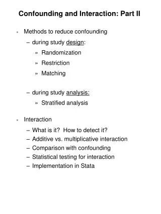
Confounding and Interaction: Part II. Methods to reduce confounding during study design : Randomization Restriction Matching during study analysis: Stratified analysis Interaction What is it? How to detect it? Additive vs. multiplicative interaction Comparison with confounding

Confounding and Interaction: Part II
E N D
Presentation Transcript
Confounding and Interaction: Part II • Methods to reduce confounding • during study design: • Randomization • Restriction • Matching • during study analysis: • Stratified analysis • Interaction • What is it? How to detect it? • Additive vs. multiplicative interaction • Comparison with confounding • Statistical testing for interaction • Implementation in Stata
Confounding ANOTHER PATHWAY TO GET TO THE DISEASE (a mixing of effects) Confounder D
Methods to Prevent or Manage Confounding By prohibiting at least one “arm” of the exposure- confounder - disease structure, confounding is precluded D or D
Randomization to Reduce Confounding • Definition: random assignment of subjects to exposure (e.g., treatment) categories • All subjectsRandomize • Distribution of any variable is theoretically the same in the exposed group as the unexposed • Theoretically, can be no association between exposure and any other variable • One of the most important inventions of the 20th Century! Exposed (treatment) Unexposed
Randomization to Reduce Confounding D Explains the significant role of randomization in clinical research Randomization prevents confounding
Randomization to Reduce Confounding • All subjectsRandomize • Of course, applicable only for intervention (experimental) studies • Special strength of randomization is its ability to control the effect of confounding variables about which the investigator is unaware • Because distribution of any variable theoretically same across randomization groups • Does not, however, always eliminate confounding! • By chance alone, there can be imbalance • Less of a problem in large studies • Techniques exist to ensure balance of certain variables Exposed Unexposed
Restriction to Reduce Confounding But what if we cannot randomize? • AKA Specification • Definition: Restrict enrollment to only those subjects who have a specific value/range of the confounding variable • e.g., when age is confounder: include only subjects of same narrow age range
Restriction to Reduce Confounding D e.g., restrict on age Birth Order ? Maternal Age Down Syndrome
Restriction to Prevent Confounding • Particularly useful when confounder is quantitative in scale but difficult to measure • e.g. • Research question: Is there an association between sexual behavior and acquisition of HHV-8 infection? • Issue: Is association confounded by injection drug use? • Problem: degree of injection drug use is difficult to measure • Solution: restrict to subjects with no injection drug use, thereby precluding the need to measure degree of injection use • Cannon et. al NEJM 2001 • Restricted to persons denying injection drug use
Restriction to Reduce Confounding • Advantages: • conceptually straightforward • Disadvantages: • may limit number of eligible subjects • inefficient to screen subjects, then not enroll • “residual confounding” may persist if restriction categories not sufficiently narrow (e.g. “20 to 30 years old” might be too broad) • limits generalizability (but don’t worry too much about this) • not possible to evaluate the relationship of interest at different levels of the restricted variable (i.e. cannot assess interaction)
Matching to Reduce Confounding • A complex topic • Definition: only unexposed/non-case subjects are chosen who match those of the comparison group (either exposed or cases) in terms of the confounder in question • Mechanics depends upon study design: • e.g. cohort study: unexposed subjects are “matched” to exposed subjects according to their values for the potential confounder. • e.g. matching on race One unexposedblack enrolled for each exposedblack One unexposedasian enrolled for each exposedasian • e.g. case-control study: non-diseased controls are “matched” to diseased cases • e.g. matching on age One controlage50enrolled for each caseage50 One controlage70enrolled for each caseage70
Matching to Reduce Confounding Cohort design D or Case-control design Also illustrates a disadvantage D
Advantages of Matching 1. Useful in preventing confounding by factors which would be difficult to manage in any other way • e.g. “neighborhood” is a nominal variable with multiple values. (complex nominal variable) • e.g. Cohort study of the effect of stop light cameras in preventing motor vehicle accidents • Exposed: persons going thru stop lights with camera • Unexposed: persons going thru stop lights without camera • Outcome: accidents • Potential confounder: ambient driving practices in the neighborhood • Relying upon random sampling of unexposed persons without attention to neighborhood may result in (especially in a small study) choosing no unexposed persons from some of the neighborhoods seen in the exposed group • Even if all neighborhoods seen in the exposed group were represented in the unexposed group, adjusting for neighborhood with “analysis phase” strategies are problematic
If you chose to stratify to manage confounding, the number of strata may be unwieldy Crude Stratified Mission Sunset Richmond Marina Pacific Heights Castro And strata for Western Addition, Russian Hill, Portero Hill, Bayview, etc
Advantages of Matching 2. By ensuring a balanced number of cases and controls (in a case-control study) or exposed/unexposed (in a cohort study) within the various strata of the confounding variable, statistical precision is increased
Smoking, Matches, and Lung Cancer A. Random sample of controls Crude OR crude = 8.8 Stratified Smokers Non-Smokers OR CF+ = ORsmokers = 1.0 OR CF- = ORnon-smokers = 1.0 ORadj= 1.0 (0.69 to 1.45) B. Controls matched on smoking Smokers Non-Smokers OR CF+ = ORsmokers = 1.0 OR CF- = ORnon-smokers = 1.0 ORadj= 1.0 (0.75 to 1.34) Little known benefit of matching: Improved precision
Disadvantages of Matching 1. Finding appropriate matches may be difficult and expensive and limit sample size (e.g., have to throw out a case if cannot find a control). Therefore, the gains in statistical efficiency can be offset by losses in overall efficiency. 2. In a case-control study, factor used to match subjects cannot be itself evaluated as a risk factor for the disease. In general, matching decreases robustness of study to address secondary questions. 3. Decisions are irrevocable - if you happened to match on an intermediary factor, you have lost ability to evaluate role of exposure in question via that pathway. e.g. study of effect of sexual activity on cervical cancer. Matching on HPV status precludes ability to look at sexual activity 4. If potential confounding factor really isn’t a confounder, statistical precision will be worse than no matching. Think carefully before you match and seek advice
Strategies in the analysis phase: Stratification to Reduce Confounding • Goal: evaluate the relationship between the exposure and outcome in strata homogeneous with respect to potentially confounding variables • Each stratum is a mini-example of restriction! • CF = confounding factor Crude Stratified CF Level I CF Level 2 CF Level 3
Smoking, Matches, and Lung Cancer Crude OR crude Stratified Smokers Non-Smokers OR CF+ = ORsmokers OR CF- = ORnon-smokers • ORcrude = 8.8 • ORsmokers = 1.0 • ORnon-smoker = 1.0
Stratifying by Multiple Confounders with More than 2 Levels Crude Potential Confounders:Age and Smoking • To control for multiple confounders simultaneously, must construct mutually exclusive and exhaustive strata:
Stratifying by Multiple Potential Confounders Crude Stratified <40 smokers 40-60 smokers >60 smokers <40 non-smokers 40-60 non-smokers >60 non-smokers Each of these strata is unconfounded by age and smoking
Summary Estimate from the Stratified Analyses • After the stratum have been formed, what to do next? • Goal: Create a single unconfounded (“adjusted”) estimate for the relationship in question • e.g., relationship between matches and lung cancer after adjustment (controlling) for smoking • Process: Summarize the unconfounded estimates from the two (or more) strata to form a single overall unconfounded “summary estimate” • e.g., summarize the odds ratios from the smoking stratum and non-smoking stratum into one odds ratio
Smoking, Matches, and Lung Cancer Crude OR crude Stratified Smokers Non-Smokers OR CF+ = ORsmokers OR CF- = ORnon-smokers • ORcrude = 8.8 (7.2, 10.9) • ORsmokers = 1.0 (0.6, 1.5) • ORnon-smoker = 1.0 (0.5, 2.0) • ORadjusted = 1.0 (0.69 to 1.45)
Smoking, Caffeine Use and Delayed Conception Crude RR crude= 1.7 Stratified Heavy Caffeine Use No Caffeine Use RRcaffeine use = 0.7 RRnocaffeine use = 2.4 Is it appropriate to summarize these two stratum-specific estimates?
Underlying Assumption When Forming a Summary of the Unconfounded Stratum-Specific Estimates • If the relationship between the exposure and the outcome varies meaningfully in a clinical/biologic sense across strata of a third variable, then it is often not appropriate to create a single summary estimate of all of the strata • i.e. the assumption is that no “interaction” is present
Statistical Interaction • Definition • when the magnitude of a measure of association (between exposure and disease) meaningfully differs according to the value of some third variable • Synonyms • Effect modification • Effect-measure modification • Heterogeneity of effect • Proper terminology • e.g. Smoking, caffeine use, and delayed conception • Caffeine use modifies the effect of smoking on the risk for delayed conception. • There is interaction between caffeine use and smoking in the risk for delayed conception. • Caffeine is an effect modifier in the relationship between smoking and delayed conception.
RR = 3.0 RR = 3.0 RR = 11.2 RR = 3.0
RR = 2.5 RR = 0.72
Interaction is likely everywhere • Susceptibility to infectious diseases • e.g., • exposure: sexual activity • disease: HIV infection • effect modifier: chemokine receptor phenotype • Susceptibility to non-infectious diseases • e.g., • exposure: smoking • disease: lung cancer • effect modifier: genetic susceptibility to smoke • Susceptibility to drugs (efficacy and side effects) • effect modifier: genetic susceptibility to drug • But in practice to date, difficult to document • Genomics may change this
Smoking, Caffeine Use and Delayed Conception: Additive vs Multiplicative Interaction Crude RR crude= 1.7 RD crude= 0.07 Stratified Heavy Caffeine Use No Caffeine Use RRcaffeine use = 0.7 RDcaffeine use = -0.06 Multiplicative interaction RRnocaffeine use = 2.4 RDnocaffeine use = 0.12 Additive interaction RD = Risk Difference = Risk exposed - Risk Unexposed
Additive vs Multiplicative Interaction • Assessment of whether interaction is present depends upon the measure of association • ratio measure (multiplicative interaction) or difference measure (additive interaction) • Hence, the term effect-measure modification • Absence of multiplicative interaction typically implies presence of additive interaction Additive interaction present RR = 3.0 RD = 0.3 Multiplicative interaction absent RR = 3.0 RD = 0.1
Additive vs Multiplicative Interaction • Absence of additive interaction typically implies presence of multiplicative interaction Multiplicative interaction present Additive interaction absent RR = 1.7 RD = 0.1 RR = 3.0 RD = 0.1
Additive vs Multiplicative Interaction • Presence of multiplicative interaction may or may not be accompanied by additive interaction RR = 2.0 RD = 0.1 No additive interaction RR = 3.0 RD = 0.1 RR = 3.0 RD = 0.4 Additive interaction present RR = 2.0 RD = 0.1
Additive vs Multiplicative Interaction • Presence of additive interaction may or may not be accompanied by multiplicative interaction RR = 3.0 RD = 0.4 Multiplicative interaction present RR = 2.0 RD = 0.1 RR = 3.0 RD = 0.2 Multiplicative interaction absent RR = 3.0 RD = 0.1
Additive vs Multiplicative Interaction • Presence of qualitative multiplicative interaction is always accompanied by qualitative additive interaction Multiplicative and additive interaction both present
Additive vs Multiplicative Scales • Additive measures (e.g., risk difference): • readily translated into impact of an exposure (or intervention) in terms of number of outcomes prevented • e.g. 1/risk difference = no. needed to treat to prevent (or avert) one case of disease • or no. of exposed persons one needs to take the exposure away from to avert one case of disease • gives “public health impact” of the exposure • Multiplicative measures (e.g., risk ratio) • favored measure when looking for causal association (etiologic research)
Additive vs Multiplicative Scales • Causally related but minor public health importance • Risk ratio = 2 • Risk difference = 0.0001 - 0.00005 = 0.00005 • Need to eliminate exposure in 20,000 persons to avert one case of disease • Causally related and major public health importance • RR = 2 • RD = 0.2 - 0.1 = 0.1 • Need to eliminate exposure in 10 persons to avert one case of disease
Smoking, Family History and Cancer: Additive vs Multiplicative Interaction Crude Family History Present Stratified Family History Absent Risk ratiofamily history = 2.0 RDfamily history = 0.20 Risk rationofamily history = 2.0 RDnofamily history = 0.05 • No multiplicative interaction but presence of additive interaction • If etiology is goal, risk ratio’s may be sufficient • If goal is to define sub-groups of persons to target: • - Rather than ignoring, it is worth reporting that only 5 persons with a family history have to be prevented from smoking to avert one case of cancer
Confounding vs Interaction • Confounding • An extraneous or nuisance pathway that an investigator hopes to prevent or rule out • Interaction • A more detailed description of the relationship between the exposure and disease • A richer description of the biologic or behavioral system under study • A finding to be reported, not a bias to be eliminated
Smoking, Caffeine Use and Delayed Conception Crude RR crude = 1.7 Stratified Heavy Caffeine Use No Caffeine Use RRcaffeine use = 0.7 RRnocaffeine use = 2.4 RR adjusted = 1.4 (95% CI= 0.9 to 2.1) Here, adjustment is contraindicated When interaction is present, confoundng becomes irrelevant!
Chance as a Cause of Interaction? Are all non-identical stratum-specific estimates indicative of interaction? Crude OR crude = 3.5 Stratified Age < 35 Age > 35 ORage <35 = 3.4 ORage >35 = 5.7
Statistical Tests of Interaction: Test of Homogeneity (heterogeneity) • Null hypothesis: The individual stratum-specific estimates of the measure of association differ only by random variation (chance or sampling error) • i.e., the strength of association is homogeneous across all strata • i.e., there is no interaction • A variety of formal tests are available with the same general format, following a chi-square distribution: • where: • effecti = stratum-specific measure of assoc. • var(effecti) = variance of stratum-specifc m.o.a. • summary effect = summary adjusted effect • N = no. of strata of third variable • For ratio measures of effect, e.g., OR, log transformations are used: • The test statistic will have a chi-square distribution with degrees of freedom of one less than the number of strata
Interpreting Tests of Homogeneity • If the test of homogeneity is “significant”, this is evidence that there is heterogeneity (i.e. no homogeneity) • i.e., interaction may be present • The choice of a significance level (e.g. p < 0.05) for reporting interaction is not clear cut. • There are inherent limitations in the power of the test of homogeneity • p < 0.05 may be too conservative • One approach is to report interaction for p < 0.20 if the magnitude of differences is high enough • i.e., if it is not too complicated to report stratum-specific estimates, it is often more revealing to report potential interaction than to ignore it. • However, meaning of p value is not different than other contexts • Not a purely statistical decision
Tests of Homogeneity with Stata 1. Determine crude measure of association e.g. for a cohort study command: cs outcome-variable exposure-variable for smoking, caffeine, delayed conception: -exposure variable = “smoking” -outcome variable = “delayed” -third variable = “caffeine” command is: cs delayed smoking 2. Determine stratum-specific estimates by levels of third variable command: cs outcome-var exposure-var, by(third-variable) e.g. cs delayed smoking, by(caffeine)
. cs delayed smoking • | smoking | • | Exposed Unexposed | Total • -----------------+------------------------+---------- • Cases | 26 64 | 90 • Noncases | 133 601 | 734 • -----------------+------------------------+---------- • Total | 159 665 | 824 • | | • Risk | .163522 .0962406 | .1092233 • | Point estimate | [95% Conf. Interval] • |------------------------+---------------------- • Risk difference | .0672814 | .0055795 .1289833 • Risk ratio | 1.699096 | 1.114485 2.590369 • +----------------------------------------------- • chi2(1) = 5.97 Pr>chi2 = 0.0145 • . cs delayed smoking, by(caffeine) • caffeine | RR [95% Conf. Interval] M-H Weight • -----------------+------------------------------------------------- • no caffeine | 2.414614 1.42165 4.10112 5.486943 • heavy caffeine | .70163 .3493615 1.409099 8.156069 • -----------------+------------------------------------------------- • Crude | 1.699096 1.114485 2.590369 • M-H combined | 1.390557 .9246598 2.091201 • -----------------+------------------------------------------------- • Test of homogeneity (M-H) chi2(1) = 7.866 Pr>chi2 = 0.0050 What does the p value mean?
Report vs Ignore Interaction?Some Guidelines Is an art form: requires consideration of both clinical and statistical significance
When Assessing the Association Between an Exposure and a Disease, What are the Possible Effects of a Third Variable? No Effect Intermediary Variable: ON CAUSAL PATHWAY I C + EM _ Effect Modifier (Interaction): MODIFIES THE EFFECT OF THE EXPOSURE Confounding: ANOTHER PATHWAY TO GET TO THE DISEASE D