Random Variables
This guide explores the fundamental concepts of discrete and continuous random variables, outlining their probability distributions through functions like p(x) and f(x). It details properties of distribution functions F(x) for both types of variables and discusses significant discrete distributions such as Bernoulli, Binomial, Poisson, and Geometric distributions. Examples demonstrate how to calculate probabilities using these distributions, enhancing understanding of how to apply stochastic models in real-world situations. ###

Random Variables
E N D
Presentation Transcript
Discrete Random Variables For a discrete random variable X the probability distribution is described by the probability function p(x) = P[X = x], which has the following properties:
Continuousrandom variables For a continuous random variable X the probability distribution is described by the probability density function f(x), which has the following properties : • f(x) ≥ 0
The distribution function F(x) This is defined for any random variable, X. F(x) = P[X ≤ x] Properties • F(-∞) = 0 and F(∞) = 1. • F(x) is non-decreasing (i. e. if x1 < x2 then F(x1) ≤F(x2) ) • F(b) – F(a) = P[a < X ≤ b].
p(x) = P[X = x] =F(x) – F(x-) Here • If p(x) = 0 for all x (i.e. X is continuous) then F(x) is continuous.
For Discrete Random Variables F(x) is a non-decreasing step function with F(x) p(x)
f(x) slope F(x) x • For Continuous Random Variables Variables F(x) is a non-decreasing continuous function with To find the probability density function, f(x), one first finds F(x) then
Success (S) • Failure (F) Suppose that we have a experiment that has two outcomes These terms are used in reliability testing. Suppose that p is the probability of success (S) and q = 1 – p is the probability of failure (F) This experiment is sometimes called a Bernoulli Trial Let Then
The probability distribution with probability function is called the Bernoulli distribution p q = 1- p
We observe a Bernoulli trial (S,F)n times. Let X denote the number of successes in the n trials. Then X has a binomial distribution, i. e. where • p = the probability of success (S), and • q = 1 – p = the probability of failure (F)
Example A coin is tossed n= 7 times. Let X denote the number of heads (H) in the n = 7 trials. Then X has a binomial distribution, with p = ½ and n = 7. Thus
p(x) x
Example If a surgeon performs “eye surgery” the chance of “success” is 85%. Suppose that the surgery is perfomed n = 20 times Let X denote the number of successful surgeries in the n = 20 trials. Then X has a binomial distribution, with p = 0.85 and n = 20. Thus
p(x) x
The probability that at least sixteen operations are successful = P[X ≥ 16] = p(16) + p(17) + p(18) + p(19) + p(20) = 0.1821 + 0.2428 + 0.2293 + 0.1368 + 0.0388 = 0.8298
Other discrete distributions Poisson distribution Geometric distribution Negative Binomial distribution Hypergeometric distribution
The Poisson distribution • Suppose events are occurring randomly and uniformly in time. • Let X be the number of events occuring in a fixed period of time. Then X will have a Poisson distribution with parameter l.
Some properties of the probability function for the Poisson distribution with parameter l.
is the probability function for the Binomial distribution with parameters n and p, and we allow n→ ∞ and p →0 such that np = a constant (= lsay) then • If
Suppose Proof:
Now Now using the classic limit
Graphical Illustration Suppose a time interval is divided into n equal parts and that one event may or may not occur in each subinterval. n subintervals time interval - Event occurs X = # of events is Bin(n,p) - Event does not occur As n→∞, events can occur over the continuous time interval. X = # of events is Poisson(l)
Example The number of Hurricanes over a period of a year in the Caribbean is known to have a Poisson distribution with l = 13.1 Determine the probability function of X. Compute the probability that X is at most 8. Compute the probability that X is at least 10. Given that at least 10 hurricanes occur, what is the probability that X is at most 15?
Solution • X will have a Poisson distribution with parameter l = 13.1, i.e.
The Geometric distribution Suppose a Bernoulli trial (S,F) is repeated until a success occurs. Let X = the trial on which the first success (S) occurs. Find the probability distribution of X. Note: the possible values of X are {1, 2, 3, 4, 5, … } The sample space for the experiment (repeating a Bernoulli trial until a success occurs is: S = {S, FS, FFS, FFFS, FFFFS, … , FFF…FFFS, …} (x – 1) F’s p(x) =P[X = x] = P[{FFF…FFFS}] = (1 – p)x – 1p
P[X = x] = p(x) = p(1 – p)x – 1 = pqx – 1 Thus the probability function of X is: A random variable X that has this distribution is said to have the Geometric distribution. Reason p(1) = p, p(2) = pq, p(3) = pq2 , p(4) = pq3 , … forms a geometric series
The Negative Binomial distribution Suppose a Bernoulli trial (S,F) is repeated until k successes occur. Let X = the trial on which the kth success (S) occurs. Find the probability distribution of X. Note: the possible values of X are {k, k + 1, k + 2, k + 3, 4, 5, … } The sample space for the experiment (repeating a Bernoulli trial until k successes occurs) consists of sequences of S’s and F’s having the following properties: • each sequence will contain k S’s • The last outcome in the sequence will be an S.
A sequence of length x containing exactly k S’s SFSFSFFFFS FFFSF … FFFFFFS The last outcome is an S The # of S’s in the first x – 1 trials is k – 1. The # of ways of choosing from the first x – 1 trials, the positions for the first k – 1 S’s. The probability of a sequence containing k S’s and x – k F’s.
The Hypergeometric distribution Suppose we have a population containing N objects. Suppose the elements of the population are partitioned into two groups. Let a = the number of elements in group A and let b = the number of elements in the other group (group B). Note N = a+ b. Now suppose that n elements are selected from the population at random. Let X denote the elements from group A. (n – X will be the number of elements from group B.) Find the probability distribution of X.\
Population GroupB(b elements) Group A (a elements) N - x x sample(n elements)
The number of ways x elements can be chosen Group A . The number of ways n - x elements can be chosen Group B . Thus the probability function of X is: The total number of ways n elements can be chosen from N = a + b elements A random variable X that has this distribution is said to have the Hypergeometric distribution. The possible values of X are integer values that range from max(0,n – b) to min(n,a)


