Download
1 / 60
600 likes | 617 Views
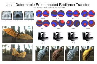
Pre-computed Radiance Transfer. Jaroslav Křivánek, KSVI , MFF UK Jaroslav.Krivanek@mff.cuni.cz. Goal. Real-time rendering with complex lighting, shadows, and possibly GI Infeasible – too much computation for too small a time budget Approaches

E N D
Pre-computed Radiance Transfer Jaroslav Křivánek, KSVI, MFF UK Jaroslav.Krivanek@mff.cuni.cz
Goal • Real-time rendering with complex lighting, shadows, and possibly GI • Infeasible – too much computation for too small a time budget • Approaches • Lift some requirements, do specific-purpose tricks • Environment mapping, irradiance environment maps • SH-based lighting • Split the effort • Offline pre-computation + real-time image synthesis • “Pre-computed radiance transfer”
R N SH-based Irradiance Env. Maps Incident Radiance (Illumination Environment Map) Irradiance Environment Map
SH-based Irradiance Env. Maps Images courtesy Ravi Ramamoorthi & Pat Hanrahan
SH-based Arbitrary BRDF Shading 1 • [Kautz et al. 2003] • Arbitrary, dynamic env. map • Arbitrary BRDF • No shadows • SH representation • Environment map (one set of coefficients) • Scene BRDFs (one coefficient vector for each discretized view direction)
SH-based Arbitrary BRDF Shading 3 • Rendering: for each vertex / pixel, do ( ) Environment map BRDF = coeff. dot product
Pre-computed Radiance Transfer • Goal • Real-time + complex lighting, shadows, and GI • Infeasible – too much computation for too small a time budget • Approach • Precompute (offline) some information (images) of interest • Must assume something about scene is constant to do so • Thereafter real-time rendering. Often hardware accelerated
Assumptions • Precomputation • Static geometry • Static viewpoint (some techniques) • Real-Time Rendering (relighting) • Exploit linearity of light transport
Relighting as a Matrix-Vector Multiply Output Image(Pixel Vector) Input Lighting (Cubemap Vector) Precomputed TransportMatrix
Problem Definition Matrix is Enormous • 512 x 512 pixel images • 6 x 64 x 64 cubemap environments Full matrix-vector multiplication is intractable • On the order of 1010 operations per frame How to relight quickly?
Outline • Compression methods • Spherical harmonics-based PRT [Sloan et al. 02] • (Local) factorization and PCA • Non-linear wavelet approximation • Changing view as well as lighting • Clustered PCA • Triple Product Integrals • Handling Local Lighting • Direct-to-Indirect Transfer
SH-based PRT • Better light integration and transport • dynamic, env. lights • self-shadowing • interreflections • For diffuse and glossy surfaces • At real-time rates • Sloan et al. 02 Env. light point light Env. lighting, no shadows Env. lighting, shadows
. . . . . . SH-based PRT: Idea Basis 16 Basis 17 illuminate result Basis 18
Relation to a Matrix-Vector Multiply • SH coefficients of transferred radiance • Irradiance • (per vertex) SH coefficients of EM (source radiance)
Idea of SH-based PRT • The L vector is projected onto low-frequency components (say 25). Size greatly reduced. • Hence, only 25 matrix columns • But each pixel/vertex still treated separately • One RGB value per pixel/vertex: • Diffuse shading / arbitrary BRDF shading w/ fixed view direction • SH coefficients of transferred radiance (25 RGB values per pixel/vertex for order 4 SH) • Arbitrary BRDF shading w/ variable view direction • Good technique (becoming common in games) but useful only for broad low-frequency lighting
Diffuse Transfer Results No Shadows/Inter Shadows Shadows+Inter
SH-based PRT with Arbitrary BRDFs • Combine with Kautz et al. 03 • Transfer matrix turns SH env. map into SH transferred radiance • Kautz et al. 03 is applied to transferred radiance
Arbitrary BRDF Results Anisotropic BRDFs Other BRDFs Spatially Varying
Outline • Compression methods • Spherical harmonics-based PRT [Sloan et al. 02] • (Local) factorization and PCA • Non-linear wavelet approximation • Changing view as well as lighting • Clustered PCA • Triple Product Integrals • Handling Local Lighting • Direct-to-Indirect Transfer
Applying Rank b: Ij • Absorbing Sj values into CiT: x x p x n Ej Sj CjT Ij p x b b x b b x n x p x n Ej Lj p x b b x n PCA or SVD factorization • SVD: Ij Ej Sj = x x p x n p x p p x n CjT diagonal matrix (singular values) n x n
Idea of Compression • Represent matrix (rather than light vector) compactly • Can be (and is) combined with SH light vector • Useful in broad contexts. • BRDF factorization for real-time rendering (reduce 4D BRDF to 2D texture maps) McCool et al. 01 etc • Surface Light field factorization for real-time rendering (4D to 2D maps) Chen et al. 02, Nishino et al. 01 • BTF (Bidirectional Texture Function) compression • Not too useful for general precomput. relighting • Transport matrix not low-dimensional!!
Local or Clustered PCA • Exploit local coherence (in say 16x16 pixel blocks) • Idea: light transport is locally low-dimensional. • Even though globally complex • See Mahajan et al. 07 for theoretical analysis • Clustered PCA [Sloan et al. 2003] • Combines two widely used compression techniques: Vector Quantization or VQ and Principal Component Analysis
Compression Example Surface is curve, signal is normal Following couple of slides courtesy P.-P. Sloan
Compression Example Signal Space
VQ Cluster normals
VQ Replace samples with cluster mean
PCA Replace samples with mean + linear combination
CPCA Compute a linear subspace in each cluster
CPCA • Clusters with low dimensional affine models • How should clustering be done? • k-means clustering • Static PCA • VQ, followed by one-time per-cluster PCA • optimizes for piecewise-constant reconstruction • Iterative PCA • PCA in the inner loop, slower to compute • optimizes for piecewise-affine reconstruction
Equal Rendering Cost VQ PCA CPCA
Outline • Compression methods • Spherical harmonics-based PRT [Sloan et al. 02] • (Local) factorization and PCA • Non-linear wavelet approximation • Changing view as well as lighting • Clustered PCA • Triple Product Integrals • Handling Local Lighting • Direct-to-Indirect Transfer
Sparse Matrix-Vector Multiplication Choose data representations with mostly zeroes Vector: Use non-linear wavelet approximation on lighting Matrix: Wavelet-encode transport rows
Non-linear Wavelet Approximation Wavelets provide dual space / frequency locality • Large wavelets capture low frequency area lighting • Small wavelets capture high frequency compact features Non-linear Approximation • Use a dynamic set of approximating functions (depends on each frame’s lighting) • By contrast, linear approx. uses fixed set of basis functions (like 25 lowest frequency spherical harmonics) • We choose 10’s - 100’s from a basis of 24,576 wavelets(64x64x6)
Non-linear Wavelet Light Approximation Wavelet Transform
Non-linear Wavelet Light Approximation ` Non-linearApproximation Retain 0.1% – 1% terms
Error in Lighting: St Peter’s Basilica Sph. Harmonics Non-linear Wavelets Relative L2 Error (%) Approximation Terms Ng, Ramamoorthi, Hanrahan 03
25 200 2,000 20,000 Output Image Comparison Top: Linear Spherical Harmonic ApproximationBottom: Non-linear Wavelet Approximation
Outline • Compression methods • Spherical harmonics-based PRT [Sloan et al. 02] • (Local) factorization and PCA • Non-linear wavelet approximation • Changing view as well as lighting • Clustered PCA • Triple Product Integrals • Handling Local Lighting • Direct-to-Indirect Transfer
SH + Clustered PCA • Described earlier (combine Sloan 03 with Kautz 03) • Use low-frequency source light and transferred light variation (Order 5 spherical harmonic = 25 for both; total = 25*25=625) • 625 element vector for each vertex • Apply CPCA directly (Sloan et al. 2003) • Does not easily scale to high-frequency lighting • Really cubic complexity (number of vertices, illumination directions or harmonics, and view directions or harmonics) • Practical real-time method on GPU
Outline • Compression methods • Spherical harmonics-based PRT [Sloan et al. 02] • (Local) factorization and PCA • Non-linear wavelet approximation • Changing view as well as lighting • Clustered PCA • Triple Product Integrals • Handling Local Lighting • Direct-to-Indirect Transfer
Problem Characterization 6D Precomputation Space • Distant Lighting (2D) • View (2D) • Rigid Geometry (2D) With ~ 100 samples per dimension ~ 1012samples total!! : Intractable computation, rendering
Factorization Approach 6D Transport = ~ 1012 samples * 4D Visibility 4D BRDF ~ 108 samples ~ 108 samples