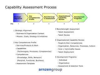
Process Capability Assessment
Process Capability Assessment. Process Capability vs. Process Control. Evaluating Process Performance Ability of process to produce parts that conform to engineering specifications (CONFORMANCE) Ability of process to maintain a state of statistical control; i.e., be within control limits


Process Capability Assessment
E N D
Presentation Transcript
Process Capability vs. Process Control • Evaluating Process Performance • Ability of process to produce parts that conform to engineering specifications (CONFORMANCE) • Ability of process to maintain a state of statistical control; i.e., be within control limits (CONTROL)
Statistical aspects • Process Control…use summary statistics from a sample (subgroup); dealing with sampling distributions, e.g., and R (LCL, UCL) Linkages Between Process Control & Process Capability • Process must be in statistical control before assessing process capability. Why? • Process Capability…dealing with individual measurements, e.g., X (LSL, USL)
Process may be in statistical control, but not capable (of meeting specifications) • Process is off-center from nominal (bias) • Process variability is too large relative to specifications (variation) • Process is both off-center and has large variation.
Upper Specification Lower Specification Relationship Between Process Variability and Product Specification (a) Process variation is small relative to the specifications so that the process mean can shift about without causing the process to degrade its capability. This will reduce the defects per million (DPM), reduce the cost of quality (COQ), and hence increase profitability.
Relationship Between Process Variability and Product Specification Upper Specification Lower Specification (b) Process variation is large relative to the specifications such that the process must remain well centered for the process capability to be maintained at a tolerable level. Variation, however, must be reduced. This will increase process capability, reduce DPMs, reduce COQ, and increase profitability.
Relationship Between Process Variability and Product Specification Upper Specification Lower Specification (c) Process variation is large relative to the specifications so that the process cannot be considered capable regardless of the process centering. Hence we have a severe and urgent problem. Process variation must be reduced drastically.
Statistical Assessment of Process Capability • Get Process in Statistical Control • Statistical Assessment (Minitab or Excel) • Construct histogram of individual measurements • Compute probability of exceeding specifications P(•) • Empirically (observed) • Mathematically: … assume N(m,s) and compute (expected) • Convert to defects per million (DPM) and sigma capability • Compute process capability indices … Cp, Cpk
Alternatives for Improving Process Capability • If bias • Recenter and recompute P(•), dpm, and sigma capability • If too much variation • Sort by 100% inspection • Widen tolerance • Use a more precise process (e.g., better or new technology) to reduce variation • Use statistical methods to identify variation reduction opportunities for existing process
Summary: Comparison of Specification Limits and Control Limits • Spec limits or tolerances for product quality characteristics are: • Characteristic of the part/item(product) in question • Based on functional design considerations • Related to/compared with an individual part measurement • Used to establish a part’s conformance to design intent
Control limits on a control chart are: • Characteristic of the process in question • Based on the process mean and variation • Dependent on sampling parameters, viz., sample size and a-risk (Type I error) • Used to identify presence/absence of special-cause variation in the process
Specification Range Variation of Distribution of Individual Product reject reject USL ~ LSL (2) (1) T -3sX(1) +3sX(1) X +3sX(2) -3sX(2) N(mX, sX) Some Common Indices of Process Capability Cp Formula Cp(1) < Cp(2)
Relationship Between Cp, DPM, and Sigma of Process (Assumes No Bias) *DPM = (Probability of Exceeding Specs) * 106
Cpk • Purpose: To promote adherence of process mean to target (nominal) value of spec. • Formulas:
LSL USL 100 190 x Example (mX-T) = bias N(130, 10) T = 145
Microeconomics of Quality: Loss Due to Variation (Taguchi) • Linking Cost of Quality Due to Bias and Variation to DPM and Process Capability in PCB Manufacture • Variation is Related to Functional Form (Distribution) of Process Output
Poor Poor Fair Fair Good Good Best Loss Function Representation of Quality for PCBs Reject (Scrap) Probability Distribution of Quality Characteristic Produced by Process Reject (Scrap) Quadratic Loss Function Quality Loss • Failure Cost @ USL = $2.40/unit • Failure Rate (Probability) = 100% X (Microns) Target (T) (Normal) USL (+8 microns) LSL (-8 microns)
Loss Function Approach • Measured loss Function: LM(X) LM(X) = k (x - T)2 where k is an unknown constant x is a value of the quality characteristic T is the target • Determining the Constant k LM(x) @ USL = k (USL - T)2 where LM(x) @ USL is a known measured cost of scrap (=Cost of a failure @ USL * failure rate (probability)) USL & T are known k = (2.40)(1.0)/(8)2 =0.0375
Total Loss Function (Measured + Hidden): LT(x) LT(x) = ak (x - T)2 where a is the hidden “cost of quality” multiplier (6 < a < 50) If we assume a = 28, then ak = 28 * 0.0375 = 1.05 • Evaluation of Expected Total Process loss: ET{L(x)} ET{L(x)} = ak {sx2 + (mx - T2)} Where sx2 is process variance and (mx - T) is process bias (mean from target)
Effect of Bias & Variation (Variance) of Process Variable on Cost of Quality in Millions of Dollars (ak = 1.05; produce 10 million units/year)
Loss Function Probability Distribution Loss ($) T LSL USL x (microns) (x -T) = 0 x = 6 ET {L(x)} = 1.05 {62 + 02} * 107 = $378 million Figure 2. Evaluation of Quality Loss Function (N(0,62))
Analysis (Figure 2.) Process Capability No. Standard Deviation from Mean (z) z = 3Cp = 3 (0.444) = 1.332 This is a 1.332 Process.
R A R M LSL -1.332 USL +1.332 Defects Per Million (dpm): Excel dpm = (1-NORMSDIST(1.332)) * 2 * 10 ^ 6 = 182,423 dpm
Loss Function Probability Distribution Loss ($) T LSL USL x (microns) (x -T) = 0 x = 2 ET {L(x)} = 1.05 {22 + 02} * 107 = $42 million Figure 3. Evaluation of Quality Loss Function (N(0,22))
Analysis (Figure 3) Process Capability No. Standard Deviation from Mean (z) z = 3Cp = 3 (1.333) = 4.000 This is a 4 Process.
Defects Per Million (dmp): Excel dpm = (1-NORMSDIST(4.000)) * 2 * 106 = 63 dpm Expected Cost Change (ECC)
(x -T) = 2 (x -T) = 2 LSL T USL x (microns) (x -T) = 2 x = 2 ET {L(x)} = 1.05 {22 + 22} * 107 = $84 million Figure 4. Quality Loss Consequences of Shifting the Process Mean Toward the Upper Specification
Analysis (Figure 4) Process Capability
No. Standard Deviation from Mean (z) ZUSL = 3 (1) = 3 ZLSL = 3(-1.67) = -5.01 Defects Per Million (dpm): Excel dpm = (1-NORMSDIST(3))+ NORMSDIST (-5.01)) * 10^6 = 1349.97 + .27 = 1350.24 Expected Cost Change (ECC)
Normal Distribution: N(0, 2.672) (Note: 3sx = 8, thus sx = 8/3 = 2.67) Loss($) LSL USL x (microns) (x -T) = 0 x = 2.67 ET{L(x)} = 1.05 {2.672 + 02} * 107 = $74.85 million
Uniform Distribution: U(0, 4.622) (Note: sx2 = (b-a)2/12 = 21.33; sx = 4.62) Loss($) LSL USL x (microns) (x -T) = 0 x = 4.62 ET{L(x)} = 1.05 {4.622 + 02} * 107 = $224.12 million
Analysis (Figure 5) Process Capability Normal Distribution Uniform Distribution (Inspection; Adjustment)
No. Standard Deviation from Mean (z) Normal Distribution Z = 3 Cp= 3 (1.000) = 3.000 This is a 3 Process. Uniform Distribution Z = 3 Cp= 3 (0.577) = 1.731 Process Defects Per Million (dmp): Excel Normal Distribution dpm = (1-NORMSDIST(3.000)* 2 * 106 = 2700 Uniform Distribution Theoretically, there are no units exceeding the specification limits; however, there are many more units further away from the target value (T) than with a normal distribution. This accounts for the higher variance (4.622 vs 2.672) and, as we shall see, higher cost of quality.
Cost of Quality Normal (N) Distribution E{L(x)} = ak {s2 + (m - T)2} = ak * 107 {2.672 + 02} = ak * 107 * 7.13 Uniform (U) Distribution E{L(x)} = ak * 107 { 4.622 + 02} = ak * 107 * 21.34 Expected Cost Change (ECC): Normal vs Uniform
Max Max T = 0 Min Min A (0, 6) B (0, 2) Process Comparison of Process (1 vs 2) (. , .) (m - T), s bias, variation
Max Max Min T = 0 Min A (0, 6) C (2, 2) Process Comparison of Process (1 vs 3) (. , .) (m - T), s bias, variation
Understanding the Differences 3s Capability Historical Standard 4s Capability Current Standard 6s Capability New Standard
Sigma Area Spelling Money Time Distance Floor space of a 1.5 misspelled $2.7 million 3 1/2 months Coast-to- s 3 small hardware words per page indebtedness per $1 per century coast trip store in a book billion in assets 45 minutes Floor space of a 1 misspelled $63,000 indebtedness of freeway 2 1/2 days per s 4 typical living word per 30 per $1 billion in driving (in century room pages in a book assets any direction) Size of the 1 misspelled $570 indebtedness A trip to 30 minutes per s 5 bottom of your word in a set of per $1 billion in the local century telephone encyclopedias assets gas station 1 misspelled 4 steps in Size of a typical word in all of the $2 indebtedness per 6 seconds per s 6 any diamond books contained $1 billion assets century direction in a small library Understanding the Differences
Understanding the Difference Suppose a process produced 294,118 units of product. If the process capability was 4s, then the defects produced could be represented by the matrix of dots given below. If the capability was 6s, only one dot would appear in the entire matrix.
Understanding the Difference 4s Capability: Defect Dots = 1849 6s Capability: Defect Dots = 1
The Inspection ExerciseTask: Count the number of times the 6th letter of the alphabet appears in the following text. The Necessity of Training Farm Hands for First Class Farms in the Fatherly Handling of Farm Live Stock is Foremost in the Eyes of Farm Owners. Since the Forefathers of the Farm Owners Trained the Farm Hands for First Class Farms in the Fatherly Handling of Farms Live Stock, the Farm Owners Feel they should Carry on with the Family Tradition of Training Farm Hands of First Class Farmers in the Fatherly Handling of Farm Live Stock Because They Believe it is the basis of Good Fundamental Farm Management.