Download
1 / 65
650 likes | 781 Views
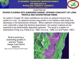
CHAPTER 26: RIVERS FLOWING INTO SUBSIDING BASINS: UPWARD CONCAVITY OF LONG PROFILE AND DOWNSTREAM FINING.

E N D
CHAPTER 26: RIVERS FLOWING INTO SUBSIDING BASINS: UPWARD CONCAVITY OF LONG PROFILE AND DOWNSTREAM FINING As noted in Chapter 25, basin subsidence can drive an upward-concave long profile of a river. An upward-concave long profile in turn implies a bed slope that decreases in the downstream direction. When sediment mixtures are transported over a bed with a slope that declines downstream, the coarser material can be expected to be preferentially deposited upstream. The result is a pattern of downstream fining (e.g. Paola et al., 1992, Cui et al., 1996; Cui and Parker, 1997). Rivers entering a (subsiding) graben in eastern Taiwan. Image from NASA website: https://zulu.ssc.nasa.gov/mrsid/mrsid.pl
CHARACTERIZATION OF PROFILE CONCAVITY AND DOWNSTREAM FINING As noted in Chapter 25, an upward-concave long profile is characterized by a bed slope S = - /x that declines downstream. Downstream fining can in turn be characterized in terms of a surface geometric geometric mean size Dsg [or corresponding arithmetic mean ] or surface median size Ds50 [or corresponding arithmetic median ] that declines in the downstream direction.
SUBSIDENCE AND PROFILE CONCAVITY: UNIFORM SEDIMENT TRANSPORTED AT CONSTANT FLOW IN A FLUME-LIKE SETTING • Before considering the case downstream fining associated with the transport of sediment mixtures in subsiding basins, it is of value to consider how a river carrying uniform sediment responds to a subsiding basin. • In a simple first analysis, the flow is considered to be constant (If = 1) and the river is taken to be flume-like, i.e. infinitely high vertical walls confining the flow to a straight channel. From Chapter 4, the appropriate form of the Exner equation of sediment conservation is • where • = bed elevation [L] x = spatial coordinate [L] t = time [T] qt = total volume bed material load per unit width [L2/T] p = bed porosity [1] = subsidence rate [L/T]
STEADY STATE UPWARD-CONCAVE LONG PROFILE IN THE PRESENCE OF SUBSIDENCE Let the subsidence rate be constant in space and time, and the upstream total volume feed rate per unit width of bed material qtf be constant in time. If the profile is allowed to evolve for a sufficient amount of time, it will achieve a steady state for which the governing equation is This equation defines a perfect balance between the creation of accomodation space to store sediment by subsidence, and filling of this accomodation space by sediment deposition.
STEADY STATE UPWARD-CONCAVE LONG PROFILE IN THE PRESENCE OF SUBSIDENCE contd. The equation subject to the boundary condition integrates to yield Note that the sediment transport rate declines linearly downstream as it is consumed in filling the accomodation space created by subsidence.
STEADY STATE UPWARD-CONCAVE LONG PROFILE IN THE PRESENCE OF SUBSIDENCE contd. The sediment transport rate qt drops to zero where x = Lmax, where The downstream variation in sediment transport rate can then be written as Here Lmax denotes the maximum length of basin that the sediment supply can fill. At this length the sediment transport rate out of the basin drops precisely to zero, i.e.
SOLUTION FOR STEADY STATE PROFILE WITH SUBSIDENCE: UNIFORM MATERIAL In Chapter 14 the following generic sediment transport relation for uniform sediment was introduced: In the above relation g denotes the acceleration of gravity, D denotes grain size, R denotes the submerged specific gravity of the sediment ( = s/ - 1), * denotes the Shields number, c* denotes a critical Shields number at the threshold of motion, s denotes the fraction of the bed shear stress that is skin friction, t is a coefficient and nt is an exponent. In Chapter 14 this relation was further reduced with the normal flow assumption and the Manning-Strickler resistance relation to the form where S = - /x = bed slope and kc = composite bed roughness height.
SOLUTION FOR STEADY STATE PROFILE WITH SUBSIDENCE: UNIFORM MATERIAL contd. Reducing the two relations below yields the following analytical solution for the steady state slope profile: Assuming = 0 at x = Lmax, the steady state bed elevation profile is given as
SAMPLE IMPLEMENTATION FOR UNIFORM MATERIAL That is, if the subsidence rate is equal to 4000 mm/year (4 m/year), the maximum basin length at which the sediment transport rate runs to zero is 52.6 km. It should be noted that a subsidence rate of 4 m/year is at least three orders of magnitude too high, whether the processes involved be either tectonic or associated with the compaction of sediment under its own weight (consolidation). The issue is resolved in succeeding slides. This notwithstanding, the results of the sample implementation are given in the next slide.
SAMPLE IMPLEMENTATION FOR UNIFORM MATERIAL contd. • = 4000 mm/year Load declines linearly downstream, slope declines downstream, bed elevation profile is upward concave.
GENERALIZATION OF THE EXNER EQUATION FOR UNIFORM SEDIMENT FROM A FLUME-LIKE SETTING TO A RIVER The Exner equation in question, i.e. the one below, requires adaptation in order to allow application to real rivers. The firstadaptation is the inclusion of a constant flood intermittency If, as first introduced in Chapter 14, in recognition of the fact that most of the time rivers are not morphologically active. Thus the Exner equation is modified to In point of fact the analysis could be modified to include entire hydrographs, as was done in Chapter 19.
GENERALIZATION OF THE EXNER EQUATION FOR UNIFORM SEDIMENT FROM A FLUME-LIKE SETTING TO A RIVER contd. The secondadaptation recognizes the fact that in an aggrading river sediment deposits not only in the channel itself, but also in a much wider belt (e.g. the floodplain or basin width, due to overbank deposition, channel migration and avulsion. Here channel width is denoted as Bc (which can be taken to be synonymous with bankfull width) and effective depositional width is denoted as Bd. Both of these are taken as constant here for simplicity. Otherwise the necessary adaptation is based on a generalization of that given in Chapter 25. The Exner equation now takes the form The above cross-section shows channel bodies resulting from migration and avulsion across a depositional surface as the river aggrades.
GENERALIZATION OF THE EXNER EQUATION FOR UNIFORM SEDIMENT FROM A FLUME-LIKE SETTING TO A RIVER contd. The thirdadaptation recognizes the fact that recognizes that much of the sediment that deposits over the depositional width can be expected to be effective “washload” in terms of the channel, i.e. sand in the case of a gravel-bed stream or mud in the case of a sand-bed stream. Here it is assumed that for each unit of bed material load deposited units of wash load are deposited. The adaptation is that given in Chapter 25. The Exner equation now takes the form Channel deposits: bed material load Overbank deposits: mixture of bed material load and wash load Architecture of fill across depositional width: view looking downstream.
GENERALIZATION OF THE EXNER EQUATION FOR UNIFORM SEDIMENT FROM A FLUME-LIKE SETTING TO A RIVER contd. The fourthadaptation recognizes the fact that channels may be sinuous. Here it is assumed that the channel has sinuosity , but that the depositional surface across which it wanders is rectangular. The appropriate modification of the Exner equation of sediment continuity is given in Chapter 25. The result is given below: note that x remains a down-channel coordinate. The above equation may be rewritten as where
REVISITATION OF THE CASE OF STEADY STATE PROFILE WITH SUBSIDENCE: RIVER VERSUS FLUME-LIKE SETTING The steady-state profile of a river with constant flow in a flume-like setting was studied in Slide 5 with the following form of the Exner equation: The generalizations for a real river encompassed in the Exner equation of the previous slide result in the following form for a steady state profile: In real rivers the effect of subsidence tends to be greatly amplified as compared with a flume-like setting with constant flow. Consider, for example the case rB = 60, If = 0.025, = 1 and = 1.5. The amplification factor is given as so that the downstream rate of loss of sediment to fill the hole created by subsidence is 800 times greater than for the case of constant flow in a flume-like setting.
THE REASONS FOR THE AMPLIFICATION OF SUBSIDENCE IN A THE CASE OF A RIVER AS COMPARED TO A FLUME-LIKE SETTING WITH CONSTANT FLOW In the example of the previous slide. the amplification factor is given as The amplification is due to the fact that rB = Bd/Bc > 1 and If < 1 in most natural cases of interest. That is a) at any given time the river deposits its sediment only in or near the river itself, whereas subsidence is assumed to be occurring at average rate over the entire depositional width, and b) the river is morphologically active only a fraction of the time, whereas the basin is assumed to be subsiding at average rate all the time. The parameters > 0 and > 1 reduce, not amplify the effective subsidence rate, but their effect us usually not nearly so profound as rB and If.
REVISITATION OF THE STEADY-STATE PROFILE contd. The solution for the steady-state profile of Slides 6 is correspondingly modified to yield the forms The solution of Slide 9 for the profiles of bed slope and elevation remain unmodified: It was noted in the previous slide that the values rB = 60, If = 0.025, = 1 and = 1.5 lead to an amplification of subsidence by a factor of 800. As a result, the above values combined with a subsidence rate of only 5 mm/year leads to exactly the same profiles as the case of a flume-like setting with constant flow and a subsidence rate of 4000 mm/year.
SAMPLE IMPLEMENTATION FOR UNIFORM MATERIAL: GENERALIZATION TO RIVER Now a subsidence rate of only 5 mm/year produces a maximum depositional length that is precisely equal to the value associated with a subsidence rate of 4000 mm/year in a flume-like setting with constant flow. The resulting profiles for bed material load qt, bed slope S and bed elevation given in the next slide are exactly the same as those given in Slide 10.
GENERALIZATION TO RIVER contd. • = 5 mm/year (but rB = 60, If = 0.025, = 1.5, = 1) Load declines linearly downstream, slope declines downstream, bed elevation profile is upward concave.
APPROACH TO STEADY STATE FOR UNIFORM MATERIAL The approach to steady state can be studied by solving the full form of the Exner equation of Slide 14, i.e. with the load equation of Slide 8, and the boundary conditions where L Lmax (so that there is always sufficient sediment to fill the basin). The initial condition is set in terms of an initial bed slope SI.
Feed sediment here! APPROACH TO STEADY STATE FOR UNIFORM MATERIAL contd. The formulation is almost identical to that of Chapter 14. The spatial grid is defined in terms of M intervals bounded by M + 1 nodes (+ a ghost node): The Exner equation discretizes to where and au is an upwinding coefficient that can be set equal to 0.5 here.
INTRODUCTION TO RTe-bookAgDegNormalSub.xls , A CALCULATOR FOR THE APPROACH TO EQUILIBRIUM IN A RIVER CARRYING UNIFORM MATERIAL AND FLOWING INTO A SUBSIDING BASIN The program RTe-bookAgDegNormalSub.xls is a descendant of RTe-bookAgDegNormal.xls. Three relatively minor changes have been implemented as follows. a) The data input worksheet “Calculator” has been modified to reflect the purpose of the code, and so as to include the following parameters: subsidence rate , ratio of depositional width to channel width rB, ratio of wash load deposited per unit bed material load and channel sinuosity . b) The code has been modified so as to include subsidence in the calculation of mass balance. c) The output has been modified to show the time evolution of not only the profile of bed elevation , but also the profiles of bed slope S and the ratio qt/qtf, where qtf denotes the volume feed rate of bed material load per unit width.
CALCULATIONS FOR A GRAVEL-BED RIVER USING RTe-bookAgDegNormalSub.xls The following input parameters were used to compute a case for a gravel-bed stream using RTe-bookAgDegNormalSub.xls. Calculations were performed for durations of 5000 and 25,000 years. Note L = 50,000 m is slightly less than Lmax.
CALCULATIONS FOR A GRAVEL-BED RIVER USING RTe-bookAgDegNormalSub.xls By 5000 years; steady state not yet achieved.
CALCULATIONS FOR A GRAVEL-BED RIVER USING RTe-bookAgDegNormalSub.xls By 5000 years; steady state not yet achieved.
CALCULATIONS FOR A GRAVEL-BED RIVER USING RTe-bookAgDegNormalSub.xls By 5000 years; steady state not yet achieved.
CALCULATIONS FOR A GRAVEL-BED RIVER USING RTe-bookAgDegNormalSub.xls In this and the next two slides Ntoprint = 4000 rather than 1000 of Slide 23 By 25,000 years; steady state achieved upward-concave elevation profile
CALCULATIONS FOR A GRAVEL-BED RIVER USING RTe-bookAgDegNormalSub.xls By 25,000 years; steady state achieved bed slope declines downstream
CALCULATIONS FOR A GRAVEL-BED RIVER USING RTe-bookAgDegNormalSub.xls By 25,000 years; steady state achieved bed material load decreases linearly downstream
NOTE ON USE OF RTe-bookAgDegNormalSub.xls The calculation below is based on exactly the same input parameters as used for Slide 27, with the exception that the initial slope SI was reduced from 0.005 to 0.002. If the initial slope SI is not sufficiently high, subsidence will overwhelm sediment deposition at the downstream end of the reach in the early stages of the calculation, and it is not possible to reach steady state while maintaining constant bed elevation at x = L. The problem is physical, not numerical. If one wishes to attain the correct final steady state using the lower initial slope, the problem can be fixed by changing the boundary condition at x = L to one of vanishing sediment transport whenever < 0 at x = L. This is done in Chapter 33. Insufficient sediment to fill basin at downstream end during evolution toward steady state
CALCULATIONS FOR A SAND-BED RIVER USING RTe-bookAgDegNormalSub.xls The following input parameters were used to compute a case for a sand-bed stream using RTe-bookAgDegNormalSub.xls. Calculations were performed for a duration of 5000 years. Note L = 50,000 m is slightly less than Lmax.
CALCULATIONS FOR A SAND-BED RIVER USING RTe-bookAgDegNormalSub.xls upward-concave elevation profile
CALCULATIONS FOR A SAND-BED RIVER USING RTe-bookAgDegNormalSub.xls bed slope declines downstream
CALCULATIONS FOR A SAND-BED RIVER USING RTe-bookAgDegNormalSub.xls bed material load decreases linearly downstream
EXNER EQUATION FOR MIXTURES INCLUDING SUBSIDENCE • The analysis for uniform sediment can be generalized to sediment mixtures, so as to allow study of downstream fining as well as profile concavity. The appropriate form for sediment conservation of mixtures in a river under conditions of subsidence was derived in Chapter 4: • In the above equation: • x denotes the streamwise coordinate [L]; • t denotes time [T]; • denotes bed elevation [L]; Fi denotes the fraction of sediment in the ith grain size range (which is characterized by size Di) in the active (surface) layer [1]; La denotes the thickness of the active (surface) layer [L]; qtT denotes the total volume bed material transport rate per unit width [L2/T]; pti denotes the fraction of material in the ith size range in the bed material load [1]; fIi denotes the interfacial fraction in the ith grain size range exchanged between surface and substrate as the bed aggrades or degrades [1]; • denotes the subsidence rate [L/T]; and p denotes the porosity of the bed deposit [1].
ADAPTATION OF THE EXNER EQUATION FOR SEDIMENT MIXTURES The Exner equation of the previous slide can be adapted to realistic rivers flowing into subsiding basins by virtue of the same steps as pursued in Slides 11 – 14 for uniform material. The result is the form where rB, If, and have the same meanings as before. Summing over all grain sizes, the relation describing the evolution of the bed is found to be: Between the two equations above, the equation for evolution of the surface size distribution is found to be:
CASE OF A STEADY STATE LONG PROFILE MAINTAINED BY A PERFECT BALANCE BETWEEN SUBSIDENCE AND DEPOSITION As outlined for the case of uniform sediment, basin subsidence creates a “hole” into which sediment can be deposited. Sediment can fill this “hole.” The long profile of the river becomes invariant in time when the deposition rate precisely balances the rate of creation of space created by subsidence. In the case of mixtures, the relevant forms of sediment conservation reduce to:
CASE OF A STEADY STATE LONG PROFILE MAINTAINED BY A PERFECT BALANCE BETWEEN SUBSIDENCE AND DEPOSITION contd. The Exner equations of the previous slide thus simplify to the following forms: The first of these equations integrates to give exactly the same forms as for uniform material: where qtTf denotes the feed rate of total bed material load.
CASE OF A STEADY STATE LONG PROFILE MAINTAINED BY A PERFECT BALANCE BETWEEN SUBSIDENCE AND DEPOSITION contd. The equation combined with and appropriate relations for flow resistance and sediment transport of mixtures, can be solved to determine the steady-state downstream variation in bed slope S and surface layer fractions Fi and thus surface geometric mean and median sizes Dsg and Ds50). In the case of sediment mixtures an analytical solution is not possible; implementation involves an iterative numerical scheme. Here an alternative scheme is pursued in terms of solution of the time-varying problem that naturally relaxes to steady state.
GRAVEL-BED RIVERS: EVOLUTION OF THE PROFILE TOWARD STEADY STATE The case of gravel-bed rivers is considered. The treatment here is an extension of that of Chapter 17. For this case the bed material load is gravel and the wash load is usually mostly sand. The relations governing the evolution toward steady state are those given in Slide 36, but with qtT→qbT and pti→ pbi, where the subscript “b” denotes bedload (Chapters 4 and 7); Bedload transport for gravel mixtures is computed using one of the methodologies introduced in Chapter 6 and implemented in Chapter 17; where u* denotes bed shear velocity and fW is specified in terms of the bedload transport relations of Parker (1990) or Wilcock and Crowe (2003) (Chapter 6).
GRAVEL-BED RIVERS: EVOLUTION OF THE PROFILE TOWARD STEADY STATE contd. Flow resistance is computed using the Manning-Strickler formulation introduced in Chapter 5 and implemented in Chapter 17; where U denotes depth-averaged flow velocity, The flow is calculated using the normal flow assumption. As in Chapter 17, the shear velocity is computed as The volume bedload transport rate per unit width qbi is then computed from the surface fractions Fi, shear velocity u*, the grain sizes Di and an appropriate bedload transport relation for mixtures as outlined in Chapter 7.
GRAVEL-BED RIVERS: EVOLUTION OF THE PROFILE TOWARD STEADY STATE contd. The interfacial exchange fractions fIi are computed from the relation of Chapter 4. In the above relation is a user-specified constant between 0 and 1 and fi denotes the fractions in the substrate. The upstream boundary conditions at x = 0 consist of a specified total volume bedload feed rate per unit width qbTf specified bedload feed fractions pfi. The downstream boundary condition at x = L consists of a fixed downstream bed elevation d (e.g. d = 0). Thus Here L must be less than Lmax, where from Slide 38
GRAVEL-BED RIVERS: EVOLUTION OF THE PROFILE TOWARD STEADY STATE contd. The initial conditions consist of specified, constant initial bed slope SI and specified initial fractions in the surface layer FIi. These initial surface fractions are taken to be the same for every node. In addition to the above parameters, it is necessary to specify the fractions in the substrate. These fractions are assumed to be the same at every node, and independent of vertical position within the bed. In a complete description, the vertical structure of the substrate would be updated whenever the river degraded into an existing deposit, and then aggraded subsequently. This step is not implemented here.
NUMERICAL IMPLEMENTATION FOR MIXTURES The formulation is identical to that of Chapter 17 except for the fact that subsidence and the parameters rB, If, and are included. As outlined in Chapter 17, M + 1 nodes bound M intervals. Sediment is fed in at a ghost node. The Exner formulations are implemented as where k is an index denoting node, and ranging from k = 1 to M + 1 (in addition to a ghost node where sediment is fed), and i is an index denoting grain size range.
INTRODUCTION TO RTe-bookAgDegNormalGravMixSubPW.xls , A CALCULATOR FOR THE APPROACH TO EQUILIBRIUM IN A GRAVEL RIVER CARRYING A MIXTURE OF SIZES AND FLOWING INTO A SUBSIDING BASIN The code in RTe-bookAgDegNormalGravMixSubPW.xls is a modestly modified version of RTe-bookAgDegNormalGravMixPW.xls, in which the modification allow for a) the inclusion of subsidence at rate and b) characterization of the river and subsiding basin in terms of the parameters If, rB, and . The code allows implementation of either the bedload relation of Parker (1990) or the one of Wilcock and Crowe (2003). The output consists of numerical data and plots for a) profiles of bed elevation, b) profiles of bed slope, c) profiles of surface geometric mean size, d) profiles of the ratio of total bedload transport rate. Calculations are presented here using: Case A) the relation of Wilcock and Crowe (2003) and widely distributed sediment feed; Case B) the relation of Wilcock and Crowe (2003) and a uniform feed sediment with the same geometric mean size as that of Case A; and Case C) the relation of Parker (1990) and the same feed distribution as in Case A.
CALCULATIONS FOR USING RTe-bookAgDegNormalGravMixSubPW.xls WITH THE GRAVEL TRANSPORT RELATION OF WILCOCK AND CROWE (2003) Case A: Sediment Mixture Percents finer
CALCULATIONS FOR USING RTe-bookAgDegNormalGravMixSubPW.xls WITH THE GRAVEL TRANSPORT RELATION OF WILCOCK AND CROWE (2003) Case A: Sediment Mixture Steady-state upward-concave profile nearly achieved
CALCULATIONS FOR USING RTe-bookAgDegNormalGravMixSubPW.xls WITH THE GRAVEL TRANSPORT RELATION OF WILCOCK AND CROWE (2003) Case A: Sediment Mixture Slope declines strongly downstream
CALCULATIONS FOR USING RTe-bookAgDegNormalGravMixSubPW.xls WITH THE GRAVEL TRANSPORT RELATION OF WILCOCK AND CROWE (2003) Case A: Sediment Mixture Surface geometric mean grain size declines downstream
CALCULATIONS FOR USING RTe-bookAgDegNormalGravMixSubPW.xls WITH THE GRAVEL TRANSPORT RELATION OF WILCOCK AND CROWE (2003) Case A: Sediment Mixture Nearly linear decline in total bedload transport rate by end of run.