Discrete Probability Distributions
Discrete Probability Distributions. Sample Space: Set of possible outcomes. For a coin toss, either get a “heads” or a “tails”. So the sample space S = {H,T}. Each outcome in the sample space will have a probability:. Random Variables. Example: Coin toss.

Discrete Probability Distributions
E N D
Presentation Transcript
Sample Space: Set of possible outcomes For a coin toss, either get a “heads” or a “tails”. So the sample space S = {H,T} Each outcome in the sample space will have a probability:
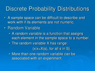
Example: S = number of girls in a two-child family: S = {BB, BG, GB, GG} and X = 0, 1, 2. Each member of the sample space can have only one numeric value x in X. But each numeric value in x in X can be associated with more than one element in the sample space S. Therefore, X is a random variable.
In the preceding example, X is a random variable with values and probabilities: * Note: Big X represents the random variable, and little x is the value of the random variable!
In the preceding example, the box is a (discrete) probability distribution with probabilities adding to 1.00. As before, with frequency distributions, probability distributions can be plotted with bar charts.
Expected Value (mean, average) μ= E(X) = Σ value(x) x probability(x)
In a sample of two-child families, the average number of girls in the family will approach 1 as the sample size increases. This graph (right) shows a computer simulation of a random variable with μ = 0 and sample size n = 250. Expected value = 0.5 x (-1) + 0.5 x (+1) = 0.
Example 2: Lottery of 1,000 tickets, with the following payout structure, has an E(x) = $1.00.
Example: Comparing the payouts and probabilities of investment portfolios .
Calculating the Variance s2 and the Standard Deviation s. Var(Y) = s2 = Σ[(y – E(Y))2 x P(y)] Or Var(Y) = s2 = Σ[P(y) x Y] – E(Y)2 SDev s = (s2)0.5
Mathematics Factorials ! n! = n x (n – 1) x (n – 2) …. x 1 Example: 6! = 6 x 5 x 4 x 3 x 2 x 1 = 720.
Example: a die is rolled exactly n = 5 times. What is the probability of rolling exactly x = 2 sixes? (Note the probability of rolling a 6 is P(six) = 1/6 = 0.166667.)
Binomial Calculators (online) http://stattrek.com/tables/binomial.aspx Or, using MS Excel, go to Formulas/More Functions/Statistical/BINOMDIST
Binomial Distribution Statistics Mean μ = np Variance σ2 = np(1 – p) Standard deviation σ = (σ2)0.5