Download
1 / 32
320 likes | 349 Views
Explore noise stability, bubbles, and half-spaces, with applications in voting schemes and graph coloring. Learn about the Peace Sign Conjecture and computational hardness. Discover influences and noise in product spaces, voting models, and robustness against noise. Dive into an invariance principle and the stability of voting schemes. Uncover the stability of voting schemes without dictatorships or juntas.

E N D
Non Linear Invariance Principles with Applications Elchanan Mossel U.C. Berkeley http://stat.berkeley.edu/~mossel
Lecture Plan • Background: Noise Stability in Gaussian Spaces • Noise := Ornstein-Uhlenbeck process. • Bubbles and half-spaces. • Double Bubbles and the “Peace Sign” Conjecture. • An invariance principle • Half-Spaces = Majorities are stablest • Peace-signs = Pluralities are stablest? • Voting schemes. • Computational hardness of graph coloring.
Gaussian Noise • Let 0 1 and f, g : Rn Rm. • Define <f, g> := E[<f(N) , g(M) >], where N,M ~ Normal(0,I) with E[Ni Mj] = (i,j). • For sets A,B let: <A,B> := <1A,1B> • Let n := standard Gaussian volume • Let n := Lebsauge measure. • Let n-1, n-1 := corresponding (n-1)-dims areas.
Some isoperimetric results • I. Ancient: Among all sets withn(A) = 1the minimizer ofn-1( A)is A = Ball. • II. Recent (Borell, Sudakov-Tsierlson 70’s) Among all sets withn(A) = athe minimizer ofn-1( A)is A=Half-Space. • III.More recent (Borell 85): For all,among all sets with (A) = a the maximizer of <A,A> is given by A =Half-Space.
Thm1 (“Double-Bubble”): • Among all pairs of disjoint sets A,Bwith n(A) = n(B) = a, the minimizer of n-1( A B) is a “Double Bubble” • Thm2(“Peace Sign”): • Among all partitions A,B,C ofRnwith (A) = (B) = (C) = 1/3 , the minimum of ( A B C) is obtained for the “Peace Sign” • 1.Hutchings, Morgan, Ritore, Ros. + Reichardt, Heilmann, Lai, Spielman 2. Corneli, Corwin, Hurder, Sesum, Xu, Adams, Dvais, Lee, Vissochi Double bubbles
The Peace-Sign Conjecture • Conj: • For all 0 1, • all n 2 • The maximum of • <A, A> + <B, B> + <C, C> • among all partitions (A,B,C) of Rnwith n(A) = n(B) = n(C) = 1/3 is obtained for • (A,B,C) = “Peace Sign”
Lecture Plan • Background: Noise Stability in Gaussian Spaces • Noise := Ornstein-Uhlenbeck operator. • Bubbles and half-spaces. • Double Bubbles and the “Peace Sign” Conjecture. • An invariance principle • Half-Spaces = Majorities are stablest • Peace-signs = Pluralities are stablest? • Voting schemes. • Computational hardness of graph coloring.
Influences and Noise in product Spaces • Let X be a probability space. • Let f L2(Xn,R). Thei’th influence of f is given by: • Ii(f) := E[ Var[f | x1,…,xi-1,xi+1,…,xn] ] • (Ben-Or,Kalai,Linial, Efron-Stein 80s) • Given a reversible Markov operator T on X and • f, g: Xn R define the T- noise form by • <f, g>T := E[f T n g] • The 2nd eigen-value(T) of T is defined by • (T) := max {|| : spec(T), < 1}
Influences and Noise in product Spaces – Example 1 • Let X = {-1, 1} with the uniform measure. • For the dictator function xj: Ii(xj) = (i,j). • For the majoritym(x) = sgn(1 i n xi) function: Ii(m) (2 n)-1/2. • Let Tbe the “Beckner Operator” on X: • Ti,j = (i,j) + (1-)/2. • T xi = xiand <xi, xi>T = . • <m, m>T ~ 2 arcsin() / • (T) = .
Definition of Voting Schemes • A population of size n is to choose between two options / candidates. • A voting scheme is a function that associates to each configuration of votes an outcome. • Formally, a voting scheme is a function f : {-1,1}n! {-1,1}. • Assume below that • f(-x1,…,-xn) = -f(x1,…,xn) • Two prime examples: • Majority vote, • Electoral college.
A voting model • At the morning of the vote: • Each voter tosses a coin. • The voters vote according • to the outcome of the coin.
A model of voting machines • Which voting schemes are more robust against noise? • Simplest model of noise: The voting machine flips each vote independently with probability . • <f, f>1-2 = correlation of intended vote with actual outcome. Registered vote Intended vote 1 prob e -1 -1 prob 1 - e -1 prob e 1 1 prob 1 - e
Majority and Electoral College • <m, m> 2 arcsin / [n ] 1 – c(1-)1/2 [ 1] • for m(x) = majority(x) = sgn(i=1n xi) • Result is essentially due to Sheppard(1899): “On the application of the theory of error to cases of normal distribution and normal correlation”. • For n1/2£ n1/2 electoral college f • <f,f> 1- c (1-)1/4 [n , 1] • <f,f>-1/2 determined prob. • of Condorcet Paradox (Kalai)
An easy answer and a hard question • Noise Theorem (folklore):Dictatorship, f(x) = xi is the most stable balanced voting scheme. • In other words, for all schemes, for all f : {-1,1}n {-1,1} with E[f] = 0 it holds that <f, f> = <x1, x1> • Harder question: What is the “stablest” voting scheme not allowing dictatorships or Juntas? • For example, consider only symmetric monotonef. • More generally: What is the “stablest” voting scheme f satisfying for all voters i: Ii(f) = P[f(x1,…,xi,…,xn) f(x1,…,-xi,…,xn)] < where n and 0. X
Influences and Noise in product Spaces – Example 2 • Let X = {0,1,2} with the uniform measure. • Let Ti,j = ½ (i j) • Then (T) = ½ and • Claim (Colouring Graph): ConsiderXn as a graph where (x,y) Edges(Xn) iff xi yi for all i. • Let A,B Xn. Then <A, B>T = 0 iff there are no edges between A and B. In particular, A is an independent set iff <A, A>T = 0. • Q: How do “large” independent sets look like?
Graph Colouring – An Algorithmic Problem • Let (G) := min # of colours needed • to colour the vertices of a graph G so that no edge is monochramatic. • ApxCol(q,Q): • Given a graph G, is (G) q or (G) Q ? • This is an algorithmic problem. How hard is it? • For q=2 easy: simply check bipartiteness • For q=3, no efficient algorithms are known unless Q >|G|0.1 • Efficient := Running time that is polynomial in |G|. • Also known that (3,4) and (3,5) are NP-hard. • NP-hard := “Nobody believes polynomial time algorithms exist”. • What about (3,6) ?????
Graph Colouring – An Algorithmic Problem • In 2002, Khot introduced a family of algorithmic problems called “games”. He speculated that these problems are NP-hard. • These problems resisted multiple algorithmic attacks. • Subhash “games conjecture” • Claim: Consider {0,1,2}n as a graph G where (x,y) Edges(G) iff xi yi for all i. • Let Q > 3. Suppose that such that for all n if there are no edges between A and B {0,1,2}n (<A,B>T = 0) and |A|,|B| > 3n/Q then there exists ani such that Ii(A) > and Ii(B) > . • Then ApxColor(3,Q) is NP hard.
[u] Graph Colouring – An Algorithmic Problem u
Influences and Noise in product Spaces – Example 3 • Let X = {0,1,2} with the uniform measure. • Let 0, 1, 2 = (1,0,0), (0,1,0),(0,0,1) R3. • Let d : Xn R3 defined by d(x) := x(1) • Let p : Xn R defined by p(x) = y • where yis the most frequent value among the xi. • Ii(d) = 2/3 (i,1);Ii(p) c n-1/2. • For 0 1, let T be the Markov operator on X defined by Ti,j = (i,j) + (1-)/3. • <d, d>T = Var(d).
Gaussian Noise Bounds • Def: For a, b, [0,1] , let • (a, b, r) := sup {< F,G > | F,G R, [F] = a, [G] = b} • (a, b, r) := inf {< F,G > | F,G R, [F] = a, [G] = b} • Thm: Let X be a finite space. Let T be a reversible Markov operator on Xwith = (T) < 1. • Then > 0 > 0 such that for all n and all f,g : Xn [0,1] satisfying maxi min(Ii(f), Ii(g)) < • It holds that <f, g>T(E[f], E[g], ) + and • <f, g>T(E[f], E[g], ) - • M-O’Donnell-Oleskiewicz-05 + Dinur-M-Regev-06
Example 1 • Taking T on {-1,1} defined by Ti,j = (i,j) + (1-)/2 • Thm : Claim: f : {-1,1}n {-1,1} with Ii(f) < for all i and E[f] = 0 it holds that: • <f, f>T <F, F> + where F(x) = sgn(x) • <F, F> = 2 arcsin()/ (F is known by Borell-85) • So “Majority is Stablest”: Most Stable “Voting Scheme” among low influence ones. • Weaker results obtained by Bourgain 2001. • “” tight in-approximation result for MAX-CUT. • Khot-Kindler-M-O’Donnell-05
Example 2 • Taking T on {0,1,2} defined by Ti,j = ½ (i j) • Thm Claim: > 0 > 0 s.t. if A,B {0,1,2}n have no edges between them and P[A], P[B] then • There exists an i s.t. Ii(A), Ii(B) . • Proof follows from Borell-85 showing (,,1/2) > 0. • Claim Hardness of approximation result for graph-colouring: • “For any constant K, it is NP hard to • colour 3-colorable graphs using K colours”. • Dinur-M-Regev-06
Example 3 • Taking T on {0,1,2} defined by Ti,j = (i,j) + (1-)/3 • Recall: 0,1,2 = (1,0,0),(0,1,0),(0,0,1) • Thm + “Peace Sign Conjecture” • Claim: (“Plurality is Stablest”): • f : {0,1,2}n {0,1,2} with E[f] = (1/3,1/3,1/3) and Ii(f) < for all i, it holds that • <f, f>T limn <p , p>T + , where • p is the plurality function on n inputs (“Plurality is Stablest”) • Claim “Optimal Hardness of approximation result” for MAX-3-CUT.
More results • More applied results use Noise-Stability bounds: • Social choice: Kalai (Paradoxes). • Hardness of approximation: • Dinur-Safra, Khot, Khot-Regev, Khot-Vishnoy etc.
Gaussian Noise Bounds • Def: For a, b, [0,1] , let • (a, b, r) := sup {< F,G > | F,G R, [F] = a, [G] = b} • (a, b, r) := inf {< F,G > | F,G R, [F] = a, [G] = b} • Thm: Let X be a finite space. Let T be a reversible Markov operator on Xwith = (T) < 1. • Then > 0 > 0 such that for all n and all f,g : Xn [0,1] satisfying maxi min(Ii(f), Ii(g)) < • It holds that <f, g>T(E[f], E[g], ) + and • <f, g>T(E[f], E[g], ) - • M-O’Donnell-Oleskiewicz-05 + Dinur-M-Regev-06
Gaussian Noise Bounds • Proof Idea: • Low influence functions are close to functions in L2() = L2(N1,N2,…). • Let H[a,b] be: • n{ f : Xn [a, b] | i: Ii(f) < , E[f] = 0, E[f2] = 1} • Then: H ““ {f L2() : E[f] =0, E[f2] = 1, a f b} • noise forms in H [a,b] ~ noise forms of [a, b] bounded functions in L2()
An Invariance Principle • For example, we prove: • Invariance Principle [M+O’Donnell+Oleszkiewicz(05)]: • Let p(x) = 0 < |S| · k aSi 2 S xi be a degree k multi-linear polynomial with |p|2 = 1 and Ii(p) for all i. • Let X = (X1,…,Xn) be i.i.d. P[Xi = 1] = 1/2 . • N = (N1,…,Nn) be i.i.d. Normal(0,1). • Then for all t: • |P[p(X) · t] - P[p(N)· t]| · O(k 1/(4k)) • Note: Noise form “kills” high order monomials. • Proof works for any hyper-contractive random vars.
Invariance Principle – Proof Sketch • Suffices to show that 8 smooth F (sup |F(4)| · C ),E[F(p(X1,…,Xn)] is close to E[F(p(N1,…,Nn))].
Invariance Principle – Proof Sketch • Write: p(X1,…,Xi-1, Ni, Ni+1,…,Nn) = R + Ni S • p(X1,…,Xi-1, Xi, Ni+1,…,Nn) = R + Xi S • F(R+Ni S) = F(R) + F’(R) Ni S + F’’(R) Ni2 S2/2 + F(3)(R) Ni3 S3/6 + F(4)(*) Ni4 S4/24 • E[F(R+ Ni S)] = E[F(R)] + E[F’’(R)] E[Ni2] /2 + E[F(4)(*)Ni4S4]/24 • E[F(R + Xi S)] = E[F(R)] + E[F’’(R)] E[Xi2] /2 + E[F(4)(*)Xi4 S4]/24 • |E[F(R + Ni S) – E[F(R + Xi S)| C E[S4] • But, E[S2] = Ii(p). • And by Hyper-Contractivity, E[S4] 9k-1 E[S2] • So: |E[F(R + Ni S) – E[F(R + Xi S) C 9k Ii2
Summary • Prove the “Peace Sign Conjecture” (Isoperimetry) • “Plurality is Stablest” (Low Inf Bounds) • MAX-3-CUT hardness (CS) and voting. • Other possible application of invariance principle: • To Convex Geometry? • To Additive Number Theory?