Improving Model Performance
300 likes | 314 Views
Learn about techniques to improve the performance of machine learning models, including parameter tuning and using the caret package. This article provides insights into optimizing algorithms to achieve better accuracy and results.

Improving Model Performance
E N D
Presentation Transcript
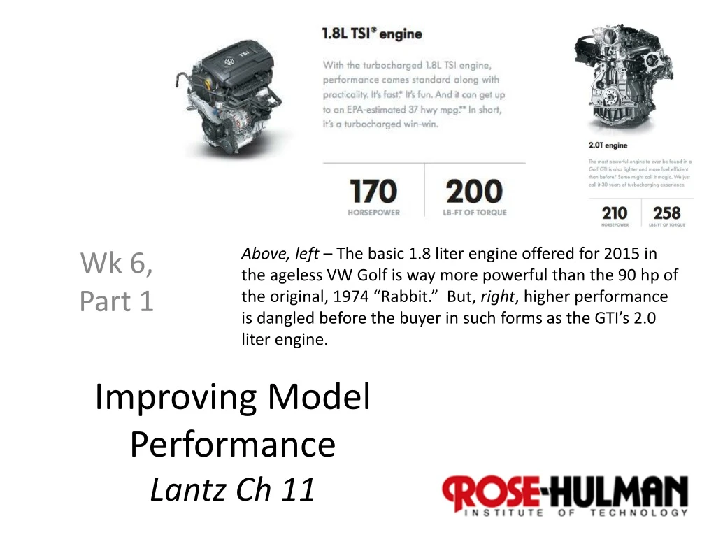
Improving Model Performance Lantz Ch 11 Above, left – The basic 1.8 liter engine offered for 2015 in the ageless VW Golf is way more powerful than the 90 hp of the original, 1974 “Rabbit.” But, right, higher performance is dangled before the buyer in such forms as the GTI’s 2.0 liter engine. Wk 6, Part 1
Reasons to go for it • The cost of spending more time perfecting an algorithm is much less than the cost of bad performance in production use of the algorithm. • The performance of the existing algorithm is unacceptable, like: • Says some poisonous mushrooms are edible, or • Misses half of the loan applicants who will default.
Let’s use those loans as an example: • In Ch 5, we used a “stock C5.0” decision tree to build the classifier for this credit data. • We attempted to improve its performance by adjusting the trials parameter to increase the number of boosting iterations. • This increased the model’s accuracy. • Called “parameter tuning.”
A general idea… • Could use parameter tuning for things other than decision trees. • We tuned the k-nearest neighbor models, searching for the best value of k. • We used a number of options for neural networks and SVMs: • Like adjusting the number of nodes, hidden layers • Choosing a different kernel function.
Typically, • Most machine learning algorithms allow you to adjust at least one parameter. • Some let you tune a lot of these. • Could lead to guessing the tuning values. • What’s a general approach to this?
Caret • We used the caret package in Ch 10. • It has tools to assist in automated tuning. • Need to ask 3 questions: • What type of machine learning model should be trained on the data? • 150 to choose from – see http://topepo.github.io/caret/modelList.htmland • Which model parameters can be adjusted, and how extensively should they be tuned? • What criteria should be used to evaluate the models to find the best candidate?
Let’s sic caret on those credit scores > library(caret) Loading required package: lattice Loading required package: ggplot2 Warning message: package ‘caret’ was built under R version 3.1.2 > set.seed(300) > m <- train(default ~ ., data = credit, method = "C5.0") Loading required package: C50 Loading required package: plyr There were 50 or more warnings (use warnings() to see the first 50)
Results of first tuning try > m C5.0 1000 samples 16 predictor 2 classes: 'no', 'yes' No pre-processing Resampling: Bootstrapped (25 reps) Summary of sample sizes: 1000, 1000, 1000, 1000, 1000, 1000, ... Resampling results across tuning parameters: model winnow trials Accuracy Kappa Accuracy SD Kappa SD rules FALSE 1 0.6847204 0.2578421 0.02558775 0.05622302 rules FALSE 10 0.7112829 0.3094601 0.02087257 0.04585890 rules FALSE 20 0.7221976 0.3260145 0.01977334 0.04512083 rules TRUE 1 0.6888432 0.2549192 0.02683844 0.05695277 rules TRUE 10 0.7113716 0.3038075 0.01947701 0.04484956 rules TRUE 20 0.7233222 0.3266866 0.01843672 0.03714053 tree FALSE 1 0.6769653 0.2285102 0.03027647 0.07001131 tree FALSE 10 0.7222552 0.2880662 0.02061900 0.05601918 tree FALSE 20 0.7297858 0.3067404 0.02007556 0.05616826 tree TRUE 1 0.6771020 0.2219533 0.02703456 0.05955907 tree TRUE 10 0.7173312 0.2777136 0.01700633 0.04358591 tree TRUE 20 0.7285714 0.3058474 0.01497973 0.04145128 Accuracy was used to select the optimal model using the largest value. The final values used for the model were trials = 20, model = tree and winnow = FALSE. Building decision trees from all 1000 samples, but taking them in different random orders.
Best results… rigged > p <- predict(m, credit) > table(p, credit$default) p no yes no 700 2 yes 0 298 > head(predict(m, credit)) [1] no yes no no yes no Levels: no yes > head(predict(m, credit, type = "prob")) no yes 1 0.9606970 0.03930299 2 0.1388444 0.86115561 3 1.0000000 0.00000000 4 0.7720279 0.22797208 5 0.2948062 0.70519385 6 0.8583715 0.14162851 We also trained on this data, so it’s just “resubstitution error.” The .73 Accuracy is closer to “how well it works on test data.”
Doing better with caret • Use kappa to optimize a boost parameter. • The trainControl() function creates configuration options – a “control object” to use with the train() function. • Defines resampling strategy like • Holdout sampling, or • K-fold cross-validation; and • Measure used to choose the best model.
On the credit scores > ctrl <- trainControl(method = "cv", number = 10, selectionFunction = "oneSE") > grid <- expand.grid(.model = "tree", + .trials = c(1, 5, 10, 15, 20, 35, 30, 35), + .winnow = "FALSE") > grid .model .trials .winnow 1 tree 1 FALSE 2 tree 5 FALSE 3 tree 10 FALSE 4 tree 15 FALSE 5 tree 20 FALSE 6 tree 35 FALSE 7 tree 30 FALSE 8 tree 35 FALSE Each row creates a candidate model
Here’s the training The winner, using oneSE > set.seed(300) > m <- train(default ~ ., data = credit, method = "C5.0", + metric = "Kappa", trControl = ctrl, tuneGrid = grid) Warning message: In Ops.factor(x$winnow) : ! not meaningful for factors > m C5.0 1000 samples 16 predictor 2 classes: 'no', 'yes' No pre-processing Resampling: Cross-Validated (10 fold) Summary of sample sizes: 900, 900, 900, 900, 900, 900, ... Resampling results across tuning parameters: trials Accuracy Kappa Accuracy SD Kappa SD 1 0.724 0.3124461 0.02547330 0.05897140 5 0.713 0.2921760 0.02110819 0.06018851 10 0.719 0.2947271 0.03107339 0.06719720 15 0.721 0.3009258 0.01969207 0.05105480 20 0.717 0.2929875 0.02790858 0.07912362 30 0.729 0.3104144 0.02766867 0.08069045 35 0.741 0.3389908 0.03142893 0.09352673 Tuning parameter 'model' was held constant at a value of tree Tuning parameter 'winnow' was held constant at a value of FALSE Kappa was used to select the optimal model using the one SE rule. The final values used for the model were trials = 1, model = tree and winnow = FALSE.
How about some meta-learning? • Combine multiple models • Complementary strengths • Could see this as learning how to learn
Create a learning “ensemble” • Out of multiple weak learners a strong learner • Have to answer 2 questions: • How are the weak learning models chosen and/or constructed? • How are the weak learners’ predictions combined to make a single final prediction?
Or, Also known as Stacking
Advantages of ensembles • Spend less time in pursuit of a single best model. • Better generalizability to future problems. • Improved performance on massive or miniscule datasets. • The ability to synthesize data from distinct domains. • The more nuanced understanding of difficult learning tasks.
One type of ensemble - Bagging • Also called Bootstrap aggregating. • Generates a number of training datasets by bootstrap sampling. • These generate a set of models using a single learning algorithm. • Their predictions are combined via: • Voting (for classification), or • Averaging (for numeric prediction).
Good for… • Unstable learners that • Change substantially with slight data changes. • These are more diverse. • So, often used with decision trees.
Credit – create & test the ensemble: > library(ipred) > set.seed(300) > mybag <- bagging(default ~ ., data = credit, nbagg = 25) > credit_pred <- predict(mybag, credit) > table(credit_pred, credit$default) credit_pred no yes no 699 2 yes 1 298
How well does it really work? > set.seed(300) > ctrl <- trainControl(method = "cv", number = 10) > train(default ~ ., data = credit, method = "treebag", trControl = ctrl) Bagged CART 1000 samples 16 predictor 2 classes: 'no', 'yes' No pre-processing Resampling: Cross-Validated (10 fold) Summary of sample sizes: 900, 900, 900, 900, 900, 900, ... Resampling results Accuracy Kappa Accuracy SD Kappa SD 0.735 0.3297726 0.03439961 0.08590462 On a par with the best-tuned C5.0 decision tree.
Beyond bags of decision trees • Caret lets you do more general bag() functions. • E.g., > str(svmBag) List of 3 $ fit :function (x, y, ...) $ pred :function (object, x) $ aggregate:function (x, type = "class") Make bags of SVM/s.
Using SVM bag on credit example: > set.seed(300) > svmbag <- train(default ~ ., data = credit, "bag", trControl = ctrl, bagControl = bagctrl) Using automatic sigma estimation (sigest) for RBF or laplace kernel Using automatic sigma estimation (sigest) for RBF or laplace kernel … > svmbag Bagged Model 1000 samples 16 predictor 2 classes: 'no', 'yes' No pre-processing Resampling: Cross-Validated (10 fold) Summary of sample sizes: 900, 900, 900, 900, 900, 900, ... Resampling results Accuracy Kappa Accuracy SD Kappa SD 0.728 0.2929505 0.04442222 0.1318101 Tuning parameter 'vars' was held constant at a value of 35 Not as good as bagged decision tree model.
Boosting • Given a number of classifiers, • Each with error rate less than 50%, • You can increase performance by combining, • Often to an arbitrary threshold, • By adding more weak learners. Like stem cells, this is a significant discovery!
What’s different here? • In boosting, • The resampled datasets are constructed specifically to generate complementary learners. • The vote is weighted based on each model’s performance, • Versus each getting an equal vote.
How boosting works • Start with an unweighted dataset • The first classifier attempts to model the outcome. • Examples it got right are less likely to appear in the dataset for the following classifier. • Examples it got wrong are more likely to appear. • So, succeeding rounds of learners are trained on data with successively more difficult examples. • Continue till the desired overall error rate is reached, or • Until performance no longer improves.
Random forests are • Ensembles of decision trees. • Combines bagging with random feature selection. • Adds diversity to the decision tree models. • After the forest is generated, the model uses a vote to combine the trees’ predictions.
Training > library(randomForest) randomForest 4.6-10 Type rfNews() to see new features/changes/bug fixes. > set.seed(300) > rf <- randomForest(default ~ ., data = credit) > rf Call: randomForest(formula = default ~ ., data = credit) Type of random forest: classification Number of trees: 500 No. of variables tried at each split: 4 OOB estimate of error rate: 23.8% Confusion matrix: no yes class.error no 640 60 0.08571429 yes 178 122 0.59333333 A decent estimate of future performance.
Evaluating performance > ctrl <- trainControl(method = "repeatedcv", number = 10, repeats = 10) > grid_rf <- expand.grid(.mtry = c(2, 4, 8, 16)) > set.seed(300) > m_rf <- train(default ~ ., data = credit, method = rf", + metric = "Kappa", trControl = ctrl, + tuneGrid = grid_rf) • This takes a while to run! • End result – similar to boosted tree.