Forecasting numeric data with regression Lantz Ch 6
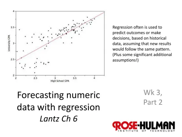
Regression often is used to predict outcomes or make decisions, based on historical data, assuming that new results would follow the same pattern. (Plus some significant additional assumptions!). Forecasting numeric data with regression Lantz Ch 6. Wk 3, Part 2. Based on a lot of math!.

Forecasting numeric data with regression Lantz Ch 6
E N D
Presentation Transcript
Regression often is used to predict outcomes or make decisions, based on historical data, assuming that new results would follow the same pattern. (Plus some significant additional assumptions!) Forecasting numeric data with regression Lantz Ch 6 Wk 3, Part 2
Based on a lot of math! • Estimating numeric relationships is important in every field of endeavor. • Can forecast numeric outcomes. • Can quantify the strength of a relationship. • Specifies relationship of a dependent variable to one or more independent variables. • Come up with a formula for the relationship, like: y = a + bx Actually, E(Y | x) = α + βx, where E(Y | x) is the expected value of Y given x. • Can be used for hypothesis testing. • Strength of the relationship
But is it even machine learning? Yes, it’s pure math. • Google say Wikipedia say… Machine learning is a scientific discipline that explores the construction and study of algorithms that can learn from data. Such algorithms operate by building a model based on inputs and using that to make predictions or decisions, rather than following only explicitly programmed instructions. Yes, it produces a new formula. Yes, though the model isn’t rich in new concepts. w Yes, this is how we use it. Yes, this one’s surely true. Maybe – you’d get the same answer every time.
Actually many kinds of regression • We’ll focus on linear. • There’s also logistic regression. • Models binary categorical outcomes. • Convert true-false to 1 or -1, etc. • We’ll discuss in this chapter. • Poisson regression. • Models integer count data. • Instead of y being linear in x,
Lantz’s Space Shuttle data > b <- cov(launch$temperature, launch$distress_ct) / var(launch$temperature) > b [1] -0.05746032 > a <- mean(launch$distress_ct) – b * mean(launch$temperature) > a [1] 4.301587 • So, y = 4.30 – 0.057x
How strong is the relationship? • This is shown by the “correlation coefficient” which goes from -1 to +1: • -1 = perfectly inverse relationship • 0 = no relationship • +1 = perfectly positive relationship > r <- cov(launch$temperature, launch$distress_ct) / (sd(launch$temperature) * sd(launch$distress_ct)) > r [1] -0.725671
Multiple linear regression • Multiple independent variables. • The model can be expressed as vectors: Y = Xβ + ε, • Where Y = the dependent variable values. • X = the array of multiple independent values. • β = the array of estimated coefficients for these, including a constant term like “a”. • ε = “error”.
Lantz’s function to return a matrix of betas > reg <- function(y, x) { + x <- as.matrix(x) + x <- cbind(Intercept = 1, x) + solve(t(x) %*% x) %*% t(x) %*% y + } • Where, • Solve() takes the inverse of a matrix • t() is used to transpose a matrix • %*% multiplies two matrices
Applied to the Shuttle data reg(y = launch$distress_ct, x = launch[3:5])[,1] Intercept temperature pressure launch_id 3.814247216 -0.055068768 0.003428843 -0.016734090
Lantz’s example – predicting medical expenses > str(insurance) 'data.frame': 1338 obs. of 7 variables: $ age : int 19 18 28 33 32 31 46 37 37 60 ... $ sex : Factor w/ 2 levels "female","male": 1 2 2 2 2 1 1 1 2 1 ... $ bmi : num 27.9 33.8 33 22.7 28.9 ... $ children: int 0 1 3 0 0 0 1 3 2 0 ... $ smoker : Factor w/ 2 levels "no","yes": 2 1 1 1 1 1 1 1 1 1 ... $ region : Factor w/ 4 levels "northeast","northwest",..: 4 3 3 2 2 3 3 2 1 2 ... $ charges : num 16885 1726 4449 21984 3867 ...
2 - Exploring the data > table(insurance$region) northeast northwest southeast southwest 324 325 364 325
Correlation matrix > cor(insurance[c("age", "bmi", "children","charges")]) age bmi children charges age 1.0000000 0.1092719 0.04246900 0.29900819 bmi 0.1092719 1.0000000 0.01275890 0.19834097 children 0.0424690 0.0127589 1.00000000 0.06799823 charges 0.2990082 0.1983410 0.06799823 1.00000000
Visualizations > pairs(insurance[c("age","bmi","children", "charges")]) > pairs.panels(insurance[c("age","bmi","children", "charges")]) Correlations Enriched scatterplots: Scatterplots: Mean values Same thing transposed. Distribution for this variable. Look like clumps.
3 - Training the model > ins_model <- lm(charges ~ age + children + bmi + sex + smoker + region, data = insurance) > ins_model Call: lm(formula = charges ~ age + children + bmi + sex + smoker + region, data = insurance) Coefficients: (Intercept) age children bmi -11938.5 256.9 475.5 339.2 sexmalesmokeryesregionnorthwestregionsoutheast -131.3 23848.5 -353.0 -1035.0 regionsouthwest -960.1 Try everything!
4 - Evaluate the results > summary(ins_model) Call: lm(formula = charges ~ age + children + bmi + sex + smoker + region, data = insurance) Residuals: Min 1Q Median 3Q Max -11304.9 -2848.1 -982.1 1393.9 29992.8 Coefficients: Estimate Std. Error t value Pr(>|t|) (Intercept) -11938.5 987.8 -12.086 < 2e-16 *** age 256.9 11.9 21.587 < 2e-16 *** children 475.5 137.8 3.451 0.000577 *** bmi 339.2 28.6 11.860 < 2e-16 *** sexmale -131.3 332.9 -0.394 0.693348 smokeryes 23848.5 413.1 57.723 < 2e-16 *** regionnorthwest -353.0 476.3 -0.741 0.458769 regionsoutheast -1035.0 478.7 -2.162 0.030782 * regionsouthwest -960.0 477.9 -2.009 0.044765 * --- Signif. codes: 0 ‘***’ 0.001 ‘**’ 0.01 ‘*’ 0.05 ‘.’ 0.1 ‘ ’ 1 Residual standard error: 6062 on 1329 degrees of freedom Multiple R-squared: 0.7509, Adjusted R-squared: 0.7494 F-statistic: 500.8 on 8 and 1329 DF, p-value: < 2.2e-16 Majority of values fell between these Significance of each coefficient How much of variation is explained by the model
5 - Improve? • Add columns for age2 and for bmi > 30, combine the latter with smoking status: > insurance$age2 = insurance$age^2 > insurance$bmi30 <- ifelse(insurance$bmi >= 30, 1, 0) > ins_model2 <- lm(charges ~ age + age2 + children + bmi + sex + bmi30*smoker + region, data = insurance) Logistic regression – create a logical variable! Then “And” it with another one we’ve been using.
Regression trees • Adapting decision trees (Ch 5) to also handle numeric prediction. • Don’t use linear regression • Make predictions based on average values at a leaf
Model trees • Do build a regression model at each leaf. • More difficult to understand. • Can be more accurate. • Compare regression models at a leaf.
Regression trees are built like decision trees • Start at root node. • Divide and conquer based on the feature that will result in the greatest increase in homogeneity after the split. • Measured by entropy, like in Ch 5 • Standard splitting criterion is standard deviation reduction (SDR):
Splitting example • P 1989 – the table > tee <- c(1,1,1,2,2,3,4,5,5,6,6,7,7,7,7) > at1 <- c(1,1,1,2,2,3,4,5,5) > at2 <- c(6,6,7,7,7,7) > bt1 <- c(1,1,1,2,2,3,4) > bt2 <- c(5,5,6,6,7,7,7,7) > sdr_a <- sd(tee) - (length(at1) / length(tee) * sd(at1) + length(at2) / length(tee) * sd(at2)) > sdr_b <- sd(tee) - (length(bt1) / length(tee) * sd(bt1) + length(bt2) / length(tee) * sd(bt2)) > sdr_a [1] 1.202815 > sdr_b [1] 1.392751 Standard deviation reduced more here, so use split B
Let’s estimate some wine quality, using a regression tree! > str(wine) 'data.frame': 4898 obs. of 12 variables: $ fixed.acidity : num 6.7 5.7 5.9 5.3 6.4 7 7.9 6.6 7 6.5 ... $ volatile.acidity : num 0.62 0.22 0.19 0.47 0.29 0.14 0.12 0.38 0.16 0.37 ... $ citric.acid : num 0.24 0.2 0.26 0.1 0.21 0.41 0.49 0.28 0.3 0.33 ... $ residual.sugar : num 1.1 16 7.4 1.3 9.65 0.9 5.2 2.8 2.6 3.9 ... $ chlorides : num 0.039 0.044 0.034 0.036 0.041 0.037 0.049 0.043 0.043 0.027 ... $ free.sulfur.dioxide : num 6 41 33 11 36 22 33 17 34 40 ... $ total.sulfur.dioxide: num 62 113 123 74 119 95 152 67 90 130 ... $ density : num 0.993 0.999 0.995 0.991 0.993 ... $ pH : num 3.41 3.22 3.49 3.48 2.99 3.25 3.18 3.21 2.88 3.28 ... $ sulphates : num 0.32 0.46 0.42 0.54 0.34 0.43 0.47 0.47 0.47 0.39 ... $ alcohol : num 10.4 8.9 10.1 11.2 10.9 ... $ quality : int 5 6 6 4 6 6 6 6 6 7 ...
Decide how much to use for training > wine_train <- wine[1:3750,] > wine_test<- wine[3751:4898,] > install.packages("rpart") > library(rpart) As usual, there’s a package to install.
3 – Training the model (of the regression tree) > m.rpart <- rpart(quality ~ ., data = wine_train) > m.rpart n= 3750 node), split, n, deviance, yval * denotes terminal node 1) root 3750 2945.53200 5.870933 2) alcohol< 10.85 2372 1418.86100 5.604975 4) volatile.acidity>=0.2275 1611 821.30730 5.432030 8) volatile.acidity>=0.3025 688 278.97670 5.255814 * 9) volatile.acidity< 0.3025 923 505.04230 5.563380 * 5) volatile.acidity< 0.2275 761 447.36400 5.971091 * 3) alcohol>=10.85 1378 1070.08200 6.328737 6) free.sulfur.dioxide< 10.5 84 95.55952 5.369048 * 7) free.sulfur.dioxide>=10.5 1294 892.13600 6.391036 14) alcohol< 11.76667 629 430.11130 6.173291 28) volatile.acidity>=0.465 11 10.72727 4.545455 * 29) volatile.acidity< 0.465 618 389.71680 6.202265 * 15) alcohol>=11.76667 665 403.99400 6.596992 * * Means leaf node. In this case, For acidity < 0.2275 and alcohol < 10.85 (see node 2, above), quality is predicted to be 5.97.
4 – Evaluating performance > p.rpart <- predict(m.rpart, wine_test) > summary(p.rpart) Min. 1st Qu. Median Mean 3rd Qu. Max. 4.545 5.563 5.971 5.893 6.202 6.597 > summary(wine_test$quality) Min. 1st Qu. Median Mean 3rd Qu. Max. 3.000 5.000 6.000 5.901 6.000 9.000 We’re close on predicting, for middle-of-the-road wines
How far off are we, on average? • Lantz’s “mean absolute error” function: > MAE <- function(actual, predicted) { + mean(abs(actual - predicted)) + } > MAE(p.rpart, wine_test$quality) [1] 0.5872652 > mean(wine_train$quality) [1] 5.870933 > MAE(5.87, wine_test$quality) [1] 0.6722474 We’re off by only 0.59 on average, out of 10. Great, huh? But the average rating was 5.87. If we’d guessed that for all of them, we’d only have been off by 0.67 on average!
5 - Ok, then let’s try a Model tree • Same wine, different training algorithm: > m.m5p <- M5P(quality ~., data = wine_train) > m.m5p M5 pruned model tree: (using smoothed linear models) alcohol <= 10.85 : | volatile.acidity <= 0.238 : | | fixed.acidity <= 6.85 : LM1 (406/66.024%) | | fixed.acidity > 6.85 : | | | free.sulfur.dioxide <= 24.5 : LM2 (113/87.697%) | | | free.sulfur.dioxide > 24.5 : | | | | alcohol <= 9.15 : | | | | | citric.acid <= 0.305 : | | | | | | residual.sugar <= 14.45 : | | | | | | | residual.sugar <= 13.8 : | | | | | | | | chlorides <= 0.053 : LM3 (6/77.537%) | | | | | | | | chlorides > 0.053 : LM4 (13/0%) | | | | | | | residual.sugar > 13.8 : LM5 (11/0%) | | | | | | residual.sugar > 14.45 : LM6 (12/0%) | | | | | citric.acid > 0.305 : | | | | | | total.sulfur.dioxide <= 169.5 : … Alcohol is still the most important split. Nodes terminate in a linear model, not in a numeric prediction of quality.
The leaf node linear models: • LM1, for example… LM num: 1 quality = 0.266 * fixed.acidity - 2.3082 * volatile.acidity - 0.012 * citric.acid + 0.0421 * residual.sugar + 0.1126 * chlorides + 0 * free.sulfur.dioxide - 0.0015 * total.sulfur.dioxide - 109.8813 * density + 0.035 * pH + 1.4122 * sulphates - 0.0046 * alcohol + 113.1021 There are 36 of these models, one for each leaf node!
Evaluation of the results – improved? > summary(p.m5p) Min. 1st Qu. Median Mean 3rd Qu. Max. 4.389 5.430 5.863 5.874 6.305 7.437 > cor(p.m5p, wine_test$quality) [1] 0.6272973 > MAE(wine_test$quality, p.m5p) [1] 0.5463023 Slightly!
Ch 6 Errata – from 12/12 email • p 194, second paragrah : should be install.packages(“rpart”), followed by library(rpart). He put the quotes around the wrong one of these two. • p 196, middle of the page: should be install.pacakges(“rpart.plot”). He left the “.” out of that. • p 199, middle of the page: mean_abserror(5.87, wine_test$quality) should be MAE(5.87, wine_test$quality). He forgot what he called his own function!