Download
1 / 13
170 likes | 360 Views
Position, Velocity and Accleration in a Fan-Cart. Regina Bochicchio, Michelle Obama, Hillary Clinton September 11, 2013. Purpose.

E N D
Position, Velocity and Accleration in a Fan-Cart Regina Bochicchio, Michelle Obama, Hillary Clinton September 11, 2013
Purpose The first purpose of this lab was to prove or disprove the hypothesis that, for motion with increasing speed in a positive direction with constant acceleration, the magnitude and sign of the acceleration is identical to that of the slope of the velocity time graph for the motion. A second purpose was to investigate the best-fit curve for the position time graph made by the fan-cart and find out whether the coefficients of the corresponding equation represent any part of the actual motion.
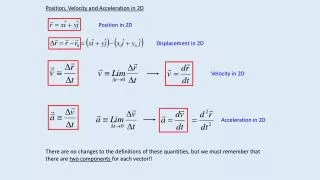
Introduction If an object moves with constant acceleration, it’s velocity will change by the same amount every second. The resulting velocity time graph is linear. The slope of the velocity time graph can be obtained by using the “rise over run” formula. Since velocity is on the vertical axis and time on the horizontal axis, this value can be calculated using the formula Δv/Δt, where the bold indicates this is a vector. The acceleration vector is defined as the rate of change of velocity (Cutnell, 2013). This value can be calculated by Δv/Δt. If this is true, then the average magnitude and sign of an object’s acceleration, should be equal to the to the slope of the velocity time graph.
Equipment EQUIPMENT: Motion detector, USB cable, computer, Logger Pro software, cart, track, fan attachment with 4 AA batteries, additional mounting bracket and elastic band (not shown below). The lab setup is shown below: motion detector Fig. 1: The track, cart with fan attachment and motion detector was set up as shown for this experiment.
Procedure • Set up the cart, ramp and motion detector as indicated in Figure 1. Make sure the ramp is level, and the fan is securely attached. • Turn on computer and start up Logger Pro. Open Logger Pro Experiments folder to Additional Physics, RealTime Physics, Mechanics, L02A1-1. • The fan cart should be no more than 20 cm in front of the motion detector at the start. The fan should be directed towards the motion detector so that the cart moves away from it on the track (see Figure 1).
Procedure (cont’d) • Turn on the fan, release the cart and collect the data. When you obtain a good data run, use Store Latest Run (from the Experiment menu). • Choose a portion of the acceleration-time graph (at least 10 samples) that is relatively horizontal. Select this portion and use the statistics feature (STAT) to find the mean acceleration. • Select the same portion of the velocity-time graph and use the linear fit function (R=) to find the slope and y-intercept of the graph. • Select the same portion of the position-time graph and use the curve-fit function to verify that a quadratic curve has a close fit to the actual data.
Velocity-time (top) and acceleration-time (bottom) graphs Fig. 2: Velocity and acceleration graphs for fan cart speeding up in positive direction. This graph shows the slope of the velocity graph taken from the linear-fit function. The value is 0.2919 m/s/s. Mean value for the corresponding section of the acceleration graph is 0.2938 m/s2 .
Error Analysis for Purpose 1 |0.2938 m/s2 - 0.2919 m/s2 |_________________________ 0.2938 m/s2 = 0.006% These numbers are very close in value!
Position as a function of time Fig. 3: Position-time graph for fan cart speeding up in positive direction. The best-fit curve for the position-time graph showing increasing speed in the positive direction is quadratic. The error term generated by the software (Root Mean Square Error) is .001, showing a very good correlation with the actual graph. The equation of this best-fit curve is: x = 0.1499t2 + 0.3273t + 0.3241
Coefficients of position-time equation Fig. 4: Position and velocity graphs for fan cart speeding up in positive direction. A comparison of the “B” term for the position-time graphs shows it to be very close to the y-intercept value of the velocity graph for the same motion: 0.3272 vs. 0.3318 m/s. This latter value indicates v0of the fancart.
Conclusions • The hypothesis given in the purpose is proven to be true. For an object moving at a constant acceleration, in a positive direction and increasing in speed, the slope of the velocity-time graph is equal to the average acceleration of the object. • The position-time graph for this motion can be represented by a quadratic equation of the form: x = At2 + Bt + C, where B represents v0, the initial velocity of the object. • This lab can be improved by investigating other motions (e.g. slowing down, moving in a negative direction) to verify the connection between the coefficient B and the initial velocity of the object.
Works Cited Cutnell, John D. and Kenneth W. Johnson. Physics. New York: John Wiley & Sons, 2013 ed.