Hebbian Model Learning
Cognitive Neuroscience and Embodied Intelligence. Hebbian Model Learning. Based on a courses taught by Prof. Randall O'Reilly , University of Colorado, Prof. Włodzisław Duch , Uniwersytet Mikołaja Kopernika and http://wikipedia.org/.

Hebbian Model Learning
E N D
Presentation Transcript
Cognitive Neuroscience and Embodied Intelligence Hebbian Model Learning Based on a courses taught by Prof. Randall O'Reilly, University of Colorado, Prof. Włodzisław Duch, Uniwersytet Mikołaja Kopernika and http://wikipedia.org/ http://grey.colorado.edu/CompCogNeuro/index.php/CECN_CU_Boulder_OReilly http://grey.colorado.edu/CompCogNeuro/index.php/Main_Page Janusz A. Starzyk
Elements: neurons, ions, channels, membranes, conductivity, impulse generation... So far Neural networks: signal transformation, filtering specific information, amplification, contrast, network stability, winner takes most (WTM), noise, network attractors... Many specific mechanisms, eg. mechano-electrical transduction of sensory signals: hair cells in the ear open ion channels with the help of proteins, functioning like springs attached to the ion channels, converting mechanical vibrations into electrical impulses. How do network configurations form which do interesting things? Learning is necessary!
How should an ideal learning system look? How does a human being learn? Learning: types Detectors (neurons) can change local parameters but we want to achieve a change in the functioning of the entire information processing network. We will consider two types of learning, requiring other mechanisms: • Learning an internal model of the environment (spontaneous). • Learning a task set by the network (supervised). • Connection of both.
Internal representations of patterns appearing in incoming signals in the environment of a given neural group. Discovering correlations between signals. Model learning positive correlation Elements of images, movements, animal behavior or emotions, we can correlate everything by creating a behavioral model. Only strong correlations are relevant, there are too many weak ones and they can be coincidental. Example: hebb_correl.proj, in Chapter 4
Select: hebb_correl.proj, in Chapter 4 Click on r.wt in the network window, after clicking on the hidden neuron we see the initialization of weights of the entire network to 0.5. Simulation Click on act in the network window, on run in the control window In effect we get binary weights => lrate = e =0.005 pright = probability of the first event Defaults changes pright =1 to 0.7
Long-Term Potentiation, LTP, was discovered in 1966 first in the hippocampus, then in the cortex. Stimulating a neuron with a current Of ~100Hz for 1 second increases synaptic efficiency by 50-100%, it's a long-term effect. Opposite effect: LTD, Long-Term Depression. Biological foundations: LTP, LTD The most common form of LTP/LTD is related to NMDA receptors. Activity of NMDA channels requires presynaptic as well as postsynaptic activity, and so is in compliance with the rule introduced by Donald Hebb in 1949, tersely summarized thus: Neurons that fire together wire together. Neurons showing simultaneous activity strengthen their bonds.
1. Mg+ ions block NMDA channels. An increase in postsynaptic potential is necessary to remove them and enable interactions with glutamate. 2. Presynaptic activity is necessary to release the glutamate, which opens NMDA channels. 3. Ca++ ions enter these channels triggering a series of chemical reactions, which are not completely tested. NMDA receptors The effect is nonlinear: small amounts of Ca++ give LTD and large amounts give LTP. Many other processes play a role in LTP. More detailed information on LTP/LTD.
From a theoretical point of view the biological mechanism LTP is not very relevant, we test only the simplest versions. Simple Hebb's rule: Dwij = e ai aj Change in weights is proportional to pre- and post-synaptic activity. xi yj=xw Hebbian Correlation Weights increase for neurons with strongly correlated activity, don't change for neurons whose activity doesn't show a correlation.
Simple Hebb's rule: Dwij = e xi yj leads to an infinite increase in weights. This can be avoided in many ways; often employed is a normalization of weights: Dwij = e (xi -wij) yj Hebb - normalization This has a biological justification: • when x and y are large we have a strong LTP, much Ca++ • when y is large but x is small we have LTD, some Ca++ • when y is small nothing happens because Mg+ ions block the NMDA channels
Hebb's mechanism allows for learning correlations. What happens if we add more postsynaptic neurons? They will learn the same correlations! If we use kWTA then output units will compete with each other. Model learning Learning = survival of the fittest (Darwin's mechanism) + specialization. Learning based on self-organization • Inhibition of kWTA: only the strongest units remain active. • Hebbian learning: the winners become even stronger. • Result: different neurons react to different signal properties.
The environment supplies a lot of information, but the signals are variable and of poor quality, the identification of objects and relationships between them isn't possible without extensive knowledge of what can be expected. We need an environmental state model biased for recognition and correct behavior; correlations are a necessary (but not sufficient) condition of causal relationships. What do we want from model learning?
This experience (bias) can also be a factor limiting recognition when we stubbornly look for old solutions in the new game. We assume that in genetic development nature worked out proven mechanisms of getting to know the world. - problem: these mechanisms aren't obvious and easy to identify. Nativists (psychologists who stress genetic influences on behavior) assume that people are born with specified knowledge about the world - this isn't genetically justified In opposition to this, a genetic record of connective structures is possible and can constitute genetically encoded knowledge (for example how to breathe or nurse) What do we want from model learning? • Expectations based on previous experience can ease adaptation to a new situation • Example – it's easier to learn a new video game if you've already played other video games and when the designers keep similar game elements
This leads to a discrepancy between the model and reality, also called the bias-variance dilemma - a precise model hinders generalization - an oversimplified model prevents correct representation A simple (parsimonious) model was preferred in the 14th century by William of Occam leading to Occam's razor – which cuts in preference of the simplest explanation of a phenomenon. What do we want from model learning? • It's more pragmatic to consider the necessity of introducing beginning knowledge through the model designer • The designer must substitute the mechanism of property selection with his own model • This is why many people avoid the introduction of preliminary assumptions (biases), preferring general machine learning mechanisms
Principal component analysis (PCA) is a mathematical technique for finding linear signal combinations with the greatest variance. Standard PCA The first neuron should learn the most important correlations, so first we calculate the correlations of its inputs averaged over time: Cik=xixkt for the first element; then for the next, but each neuron should be independent, so it should calculate orthogonal combinations. For the set of images consecutive components look like this ===============> How to do this with the help of neurons?
Let's assume that the environment is composed of diagonal lines. Let's accept a linear activation for moment t (image nr t): PCA on one neuron Let the change in weights be specified by the simple Hebb's rule: wij(t+1) = wij(t) + exi yj After presentation of all the images: The change in weights is proportional to the average of the product of the inputs/outputs. Correlation can replace average.
If the averages are zero and the variance is one then the average of the product is the correlation; the change in weights is proportional to: Hebbian Correlations Correlation: Cik=xixkt are correlations between inputs; the average of the weights changes slowly. The change in weight for input i is then the weighted average of the correlations between the activity of this input and the remaining ones. After the presentation of many images, the weights will be dominated by the strongest correlations and yj will calculate the strongest component of PCA
The two first inputs are completely correlated; the third is uncorrelated. Changes follow according to Hebb's rule for e=1. Example Let's assume that the signals have a zero average (xi=+1 the same number of times as xi=-1); for each vector x =(x1,x2,x3), y is calculated, and then the new weights. Correlated units determine the symbol and scale of the weights,and weights of these inputs grow quickly, whereas the weight of the uncorrelated input x3 decreases. The weights of unit j change in this way: w(t+1)=w(t)+Cw(t)
The simplest normalization avoiding an infinite increase in weights: Dwij = e (xi – wij) yj Erkki Oja (1982) proposed: Dwij = e (xi –yj wij) yj For one unit, after learning the weights stop changing: Dwij = 0 =e (xi –yj wij) yj Weight wij = xi /yj = xi /Skxk wkj The weight of a given input signal is then a fraction of the complete weighted activity of all the signals. This rule also leads to the calculation of the most important main component. How to calculate the other components? Normalization
How to generate the succeeding PCA components in neural networks? We numerically perform orthogonalization of successive yj but this is not easy to do with the help of a neural network. Problems of PCA • Sequential PCA orders components, from the most important to the least; this can be achieved by introducing connections between hidden neurons, but this is an artificial solution. • PCA assumes a hierarchical structure: the most important component for all images, in effect we get eg. for image analysis, successive components as chessboards with an increasing number of squares since the correlations of pixels for a large number of images disappear. • The problem with PCA can be characterized as: PCA calculates correlations in the entire input space whereas useful correlations exist in local subspaces. • Natural images create heterarchies, different combinations are equally important for different images, subsets of features relevant for certain categories are not important for differentiating others.
Conditional principal component analysis (CPCA): calculate correlations not for all features but only for these features which are present. Conditional PCA PCA functions on all features, giving orthogonal components. CPCA functions on subsets of features, ensuring that different components encode different interesting combinations of signal features, eg. edges. The competition realized with the help of kWTA will ensure the activity of different neurons for different images. In effect: encoding images => How to do this with the help of neurons?
A neuron is trained only on a subset of images with predetermined features, eg. edges slanting in a certain way. Normalized Hebb's rule: Dwij = e (xi -wij) yj The weights move in direction xi, on condition of the activity of yj. In effect the conditional probability: P(xi=1|yj=1) = P(xi|yj) = wij The weight wij = the probability that the input unit xiis active given that the receiving unit yjis also active. CPCA equations
The success of CPCA depends on the selection of a function determining the activity of neurons – an automatic determination process is possible in a few ways: self-organization or error correction. Activations averaged over time are represented by probabilities P(xi|t), P(yj|t). The change in weights for all images t appearing with P(t): Dwij = e [St (P(yj|t) P(xi|t)-P(yj|t)wij] P(t) In a state of equilibrium Dwij =0 so: wij = St P(yj|t)P(xi|t)P(t)/ St P(yj|t)P(t) = St P(yj,xi,t)/ St P(yj,t) = P(xi ,yj)/P(yj) = P(xi|yj) Weight wij = conditional probability xiunder condition yj. How to biologically justify normalization? Probabilistic interpretation
Normalized Hebb's rule: Dwij = e (xi -wij) yj Let's assume that the weights are wij ~0.5, there are then 3 possibilities: 1. xi , yj~1 (a strong pre- and postsynaptic activity), so xi > wij, weights increase, so we have LTP, as in NMDA channels. 2. yj~1 but xi < wij, weight decrease, we have LTD, a weak input signal will suffice to unblock the Mg+ ion of NMDA channel. A strong postsynaptic activity can also unblock other voltage dependent channels and introduce a small amount of Ca++. 3. Activity yj~0 doesn't give any changes, voltage channels and NMDA aren't active. Learning happens faster for small wij, because xi < wij more often. Qualitatively consistent with observations of weight saturation. Biological interpretation
Select: hebb_correl.proj, in Chapter 4 Description: Chapter 4. 6 Look at Events Evt Label, and within this FreqEvent is 1 for Right and 0 for Left Change in weight values: Graph_log lrate = 0.005, try 0.1 Change p_right from 1 to 0.7 and to 0.5 Change Env_type from One_line to Three_lines and p_right=0.7 Notice that the weights are becoming small, diffuse, because the conditional probabilities for images learning entire categories are becoming small; the output unit contributes to this because it has a small selectivity. Simulations
CPCA weights are not very selective, don't lead to image differentiation – they don't have dynamic range; for typical situations P(xi|yj) is small, but we want it around 0.5. Solution: renormalization of weights and contrast enhancement. Normalization of weights in CPCA Normalization: uncorrelated signals should have a weight of 0.5, but in simulations with seldom appearing signals xi approach a value of a~0.1-0.2. Let's factorize the weight change into two terms: Dwij = e (xi -wij) yj= e [(1-wij) xi yj+(1-xi)(0-wij)yj] The first term causes an increase in weights in the direction of 1, the second causes a decrease in the direction of 0; if we want to maintain average weights around 0.5 we must increase the first term, eg. : Dwij = e [(0.5/a-wij) xi yj+(1-xi)(0-wij)yj] The linear correlation is still wij = P(xi|yj)0.5/a .The simulator has a parameter savg_cor[0,1] determining the degree of normalization
Contrast in CPCA Instead of a linear weight change we want to ignore weak correlations and strengthen strong correlations – to increase the contrast between interesting aspects of signals and those that are not. This increases the simplicity of the connections (the weak ones can be skipped) and accelerates the learning process, helping the weights decide what to do. Contrast enhancement: instead of a linear weight change use a sigmoidal one: Two parameters: gain gand offset q. Where q>1 imposes higher threshold Attention: this is a scaling of individual weights not of activations!
Select: hebb_correl.proj, in Chapt. 4 Description: Chapt. 4. 6 Change Env_type from One_line to Five_lines and p_right=0.7 For these lines CPCA gives identical weights around 0.2. Change the normalization, setting savg_cor=1 The weights should be around 0.5 The parameter savg_cor allows us to influence the number of features used by the hidden units. Contrast: set wt_gain=6 instead of 1, PlotEffWt will show the curve of effective weights. Influence on learning: for Three_lines, savg_cor=1 Change wt_off from 1 to 1.25 Simulations