Download

1 / 37
370 likes | 416 Views
Convergence Time to Nash Equilibria in Load Balancing. Eyal Even-Dar, Tel-Aviv University Alex Kesselman, Tel-Aviv University Yishay Mansour, Tel-Aviv University. Game Theory and CS. AI: Machine Learning Reinforcement learning Multiple agents Communication Networks:

E N D
Convergence Time to Nash Equilibriain Load Balancing Eyal Even-Dar,Tel-Aviv University Alex Kesselman,Tel-Aviv University Yishay Mansour,Tel-Aviv University
Game Theory and CS • AI: • Machine Learning • Reinforcement learning • Multiple agents • Communication Networks: • Huge networks with little control • Futuristic control mechanisms • CS Theory
Motivation: Internet • Diverse set of users • Very large scale system • Extremely hard to optimize • Selfish goals and behavior • Relative anonymity • Consider game theory • Non-cooperative players
Routing: Motivating example • Each source can select a route • Source Goal: Minimize latency • Solution concept: Nash Eq. • Global Goal: Maximize utilization • Coordination Ratio • How bad can Nash Eq. be?
Job Scheduling • Classic setting: • Centralize control • Optimize an objective function • minimize MAX load • Full cooperation • Game theory setting: • Congestion and Potential games • Each job optimizes its objective • Load of the machine it selects.
What are we after? • Convergence TIME to reach a Nash Eq. • Major issue • For implementation • Understanding the constraints • Theoretical interest. • Non Issue (here) • The quality of the resulting Nash.
Model: Jobs and Machines • Job Scheduling: • m machines • n jobs • Machine Model: • Machine Mi has speed Si • m machines ands speeds in [Smin , Smax] • Jobs Model: • Unrelated: job J a weight wk(J) on Mk • Otherwise: job J a weight w(J) • Restricted: job J can be assign to M in R(J)
Model: Weights and Load • Weights: • Total sum of weights W • Maximum weight wmax • integer versus arbitrary weights. • Discrete weights: K different weights • Load Model: • Machine Mi at time t: • Bi(t) = jobs running on Mi • Li(t) = Σj in Bi(t)wi (j) ; Lmax = MAX Li • Ti(t) = Li(t) / Si ; Tmax = MAX Ti
M1 Machines L4 B2 M2 M3 M4
Model: Nash Equilibrium • No job can move and lower its load. • For a job J at Mi • For any Mj • If J moves to Mj • Then Ti Tj + wj(J)/Sj • The load after the move is not lower than before!
Model: Migration • Elementary step system (ESS): • Only one job moves at a time. • Job’s aim: minimize its observed load • A(t) = jobs wanting to move at time t • Job’s move • improvement • best reply • Scheduler: • arbitrary; • Specific: random; FIFO; Max Weight; Max Load
Our motivation • Study the time it takes the system to converge. • Arbitrary schedule: • Universal guarantee. • Specific Schedule: • Optimize convergence
Results overview • Unrelated Machines • Always converges • Identical Machines: • Arbitrary [Min Weight]: • Lower bound (Exponential in m) • Max Weight: n • FIFO: (n2) • Random: O(n2)
Results Overview • Related Machines [ignore speeds]: • Arbitrary: O(W2) • Max Load: O(W√m + n (wmax)2) • Restricted and unit weight Jobs: • strategy with O( m n ) [ideas similar to Milchtaich ’96] • Discrete weights: • wmax = O( K n4K )
Max Job First M1 M2 M3 M4
Min Job First M1 M2 M3 M4
Upper bound: Unrelated • Claim: No global system state occurs twice. • Lexicographic sorted order of states • 90, 100, 20, 1, 3, 100, 5, 2, 90, 90, 90 • 100, 100, 90, 90, 90,90, 20, 5, 3, 2, 1 • improvement step -> lower order • move from load 90 to 1 • 90 lowers to 85 • 1 increases to 89 • 100, 100, 85, 90, 90,90, 20, 5, 3, 2, 89 • 100, 100, 90, 90,90,89,85, 20, 5, 3, 2
Upper bound: Unrelated • Convergence bounds: • Number of state • General: mn • K Weights:
Upper Bound: Unrelated • Integer Weights: • Potential Function: • Each move the Potential reduces: • Consider a move from Mi to Mk
Upper Bound: Unrelated • Convergence bound: • Arbitrary: • Let W= J maxj wj(J) • Initially 4W max{P(t)}, • Each move drops by at least 2 • Bound O(4W) • Max Load Machine: • Initially, each move drops by P(t)/2m • O(mW + m 4W/m+ wmax)
1 m 1 m 2 2 1 m 2 Lower Bound: Two identical Machines Theorem: Min Job First requires at least (n2) steps to converge.
Lower bound: Identical Machines • K distinct weights • Each weight has n/K=r jobs • weight wi+1 >> wi • m=K+1 Machines numbered 0 to K • Initial configuration • Machine Mi has all jobs of weight wi • Scheduler: Min job First • Each move of job wi creates an avalanche
Identical Machines • Lower Bound • duration of phase i is ri/(2 i!) • lower bound (n/k)k/(2 k!) • Upper bound • arbitrary schedule • upper bound (n/k +1)k
Upper Bound : Identical machinesMax Weight + Best response Theorem: Max Weight + Best response: stabilizes in at most n moves Claim: Using Best Response in identical machine, after job J stabilizes it will move only after a larger job reached its machine.
Upper Bound : Identical machinesMax Weight + Best response • Consider job J which moved to Mi • At time of move its stable • Job J’ moves to Mk • J’ improved • J did not want to move to Mk • Job J’ moves to Mi and w(J’) < w(J) • This was the best response of J’
Upper Bound: Related Machines • Potential function: • Smin =1 and wmin =1 • Lemma • When a job of size w move from Mu to Mv Pr(t+1)-Pr(t) = 2 w (Tv(t+1)-Tu(t)) < 0
Upper Bound: Related • Theorem: • Related & Restricted assignments • -Nash: O(W2/) • Initial potential =O(W2) • Each move improves by • Nash [integer weights]: O(W2 (Smax)2) • Smallest = O(1/ (Smax)2)
Upper Bound: Related • Theorem: • Max Load [Related & unrestricted] • -Nash
Discrete Integer Weights • Bound the maximum weight • A priori, unbounded • Two weights: wmaxn • Beyond two: much more tricky! • Define equivalence of weights • Same “relative size” for two assignments • Viewit as an integer program • Bound solution size: K (c Smax n)4K
What’s next • Consider paths in graphs • General Load and Additive cost: • No DET Nash [LO] • Max Cost: Always converges. • General Congestion games • Personal Preferences and weights [M] • Beyond DET Nash.