Download
1 / 62
670 likes | 1.1k Views
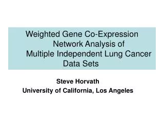
A General Framework for Weighted Gene Co-Expression Network Analysis. Steve Horvath Human Genetics and Biostatistics University of CA, LA. Content. Novel statistical approach for analyzing microarray data: weighted gene co-expression network analysis

E N D
A General Framework for Weighted Gene Co-Expression Network Analysis Steve Horvath Human Genetics and Biostatistics University of CA, LA
Content • Novel statistical approach for analyzing microarray data: • weighted gene co-expression network analysis • Empirical evidence that it matters in practice • Application 1: identifying cancer genes • Application 2: comparing chimp and human brain
Does this map tell you which cities are important? This one does! The nodes with the largest number of links (connections) are most important! **Slide courtesy of Paul Mischel and AL Barabasi
Background • Network based methods have been found useful in many domains, • protein interaction networks • the world wide web • social interaction networks • OUR FOCUS: gene co-expression networks
Scale free topology is a fundamental property of such networks (Barabasi et al) • It entails the presence of hub nodes that are connected to a large number of other nodes • Such networks are robust with respect to the random deletion of nodes but are sensitive to the targeted attack on hub nodes • It has been demonstrated that metabolic networks exhibit scale free topology at least approximately.
P(k) vs k in scale free networks P(k) • Scale Free Topology refers to the frequency distribution of the connectivity k • p(k)=proportion of nodes that have connectivity k
How to check Scale Free Topology? Idea: Log transformation p(k) and k and look at scatter plots Linear model fitting R^2 index can be used to quantify goodness of fit
Generalizing the notion of scale free topology Motivation of generalizations: using weak general assumptions, we have proven that gene co-expression networks satisfy these distributions approximately. Barabasi (1999) Csanyi-Szendroi (2004) Horvath, Dong (2005)
Checking Scale Free Topology in the Yeast Network • Black=Scale Free • Red=Exp. Truncated • Green=Log Log SFT
Gene Co-expression Networks • In gene co-expression networks, each gene corresponds to a node. • Two genes are connected by an edge if their expression values are highly correlated. • Definition of “high” correlation is somewhat tricky • One can use statistical significance… • But we propose a criterion for picking threshold parameter: scale free topology criterion.
Overview: gene co-expression network analysis Steps for constructing asimple, unweighted co-expression network • Hi • Microarray gene expression data • Measure concordance of gene expression with a Pearson correlation • C) The Pearson correlation matrix is dichotomized to arrive at an adjacency matrix. Binary values in the adjacency matrix correspond to an unweighted network. • D) The adjacency matrix can be visualized by a graph.
Our `holistic’ view…. • Weighted Network View Unweighted View • All genes are connected Some genes are connected • Connection Widths=Connection strenghts All connections are equal Hard thresholding may lead to an information loss.
Network=Adjacency Matrix • A network can be represented by an adjacency matrix, A=[aij], that encodes whether/how a pair of nodes is connected. • A is a symmetric matrix with entries in [0,1] • For unweighted network, entries are 1 or 0 depending on whether or not 2 nodes are adjacent (connected) • For weighted networks, the adjacency matrix reports the connection strength between gene pairs
Generalized Connectivity • Gene connectivity = row sum of the adjacency matrix • For unweighted networks=number of direct neighbors • For weighted networks= sum of connection strengths to other nodes
Using an adjacency function to define a network • Measure co-expression by a similarity s(i,j) in [0,1] e.g. absolute value of the Pearson correlation • Define an adjacency matrix as A(i,j) using an adjacency function AF(s(i,j)) • AF is a monotonic function from [0,1] onto [0,1] • Here we consider 2 classes of AFs • Step function AF(s)=I(s>tau) with parameter tau (unweighted network) • Power function AF(s)=sb with parameter b • The choice of the AF parameters (tau, b) determines the properties of the network.
Comparing the power adjacency functions with the step function Adjacency =connection strength Gene Co-expression Similarity
The scale free topology criterion for choosing the parameter values of an adjacency function. A) CONSIDER ONLY THOSE PARAMETER VALUES THAT RESULT IN APPROXIMATE SCALE FREE TOPOLOGY B) SELECT THE PARAMETERS THAT RESULT IN THE HIGHEST MEAN NUMBER OF CONNECTIONS • Criterion A is motivated by the finding that most metabolic networks (including gene co-expression networks, protein-protein interaction networks and cellular networks) have been found to exhibit a scale free topology • Criterion B leads to high power for detecting modules (clusters of genes) and hub genes.
Criterion A is measured by the linear model fitting index R2 Step AF (tau) Power AF (b) b= tau=
Trade-off between criterion A (R2) and criterion B (mean no. of connections) when varying the power b Power AF(s)=sb criterion A: SFT model fit R^2 criterion B: mean connectivity
Trade-off between criterion A and B when varying tau Step Function: I(s>tau) criterion A criterion B
Define a Gene Co-expression Similarity Define a Family of Adjacency Functions Determine the AF Parameters Define a Measure of Node Dissimilarity Identify Network Modules (Clustering) Relate Network Concepts to Each Other Relate the Network Concepts to External Gene or Sample Information
How to measure distance in a network? • Mathematical Answer: Geodesics • length of shortest path connecting 2 nodes • Biological Answer: look at shared neighbors • Intuition: if 2 people share the same friends they are close in a social network • Use the topological overlap measure based distance proposed by Ravasz et al (2002)
Topological Overlap leads to a network distance measure (Ravasz et al 2002) • Generalized in Zhang and Horvath (2005) to the case of weighted networks
The general topological overlap matrix N1(i) denotes the set of neighbors of node i |*| measures the cardinality We have re-interpreted the TOM measure as the “normalized” proportion of genes that are in both node neighborhoods. This allows for a straightforward generalization to “larger” neighborhoods. Yip, Horvath (2005)
Module Identification based on the notion of topological overlap • One important aim of metabolic network analysis is to detect subsets of nodes (modules) that are tightly connected to each other. • We adopt the definition of Ravasz et al (2002): modules are groups of nodes that have high topological overlap.
Steps for defining gene modules • Define a dissimilarity measure between the genes. • Standard Choice: dissim(i,j)=1-abs(correlation) • Choice by network community=1-Topological Overlap Matrix (TOM) • Used here • Use the dissimilarity in hierarchical clustering • Define modules as branches of the hierarchical clustering tree • Visualize the modules and the clustering results in a heatmap plot Heatmap
Using the TOM matrix to cluster genes • To group nodes with high topological overlap into modules (clusters), we typically use average linkage hierarchical clustering coupled with the TOM distance measure. • Once a dendrogram is obtained from a hierarchical clustering method, we choose a height cutoff to arrive at a clustering. • Here modules correspond to branches of the dendrogram TOM plot Genes correspond to rows and columns TOM matrix Hierarchical clustering dendrogram Module: Correspond to branches
Different Ways of Depicting Gene Modules Topological Overlap Plot Gene Functions We propose Multi Dimensional Scaling Traditional View 1) Rows and columns correspond to genes 2) Red boxes along diagonal are modules 3) Color bands=modules Idea: Use network distance in MDS
More traditional view of module Columns=Brain tissue samples Rows=Genes Color band indicates module membership Message: characteristic vertical bands indicate tight co-expression of module genes
Our team (module)-centric view v.s. traditional prima-donna (hub) centric view • Module view based on within module connectivity • Traditional view based on whole network connectivity In many applications, we find that intramodular connectivity is biologically and mathematically more meaningful than whole network connectivity Mathematical Facts (Horvath, Dong, Yip 2005) Hub genes are always module genes in co-expression networks. Most module genes have high connectivity.
Yeast Data Analysis Marc Carlson Findings 1) The intramodular connectivities are related to how essential a gene is for yeast survival 2) Modules are highly preserved across different data sets 3) Hub genes are highly preserved across species Within Module Analysis Prob(Essential) Connectivity k
Hub Genes Predict Survival for Brain Cancer PatientsMischel PS, Zhang B,et al, Horvath S, Nelson SF.
Module structure is highly preserved across data sets 55 Brain Tumors VALIDATION DATA: 65 Brain Tumors Messages: 1) Cancer modules can be independently validated 2) Modules in brain cancer tissue can also be found in normal, non-brain tissue. --> Insights into the biology of cancer Normal brain (adult + fetal) Normal non-CNS tissues
Gene prognostic significance Definition • Regress survival time on gene expression information using a univariable Cox regression model • Obtain the score test p-value • Gene significance=-log10(p-value) • Roughly speaking Gene significance~no of zeroes in the p-value. Goal Relate gene significance to intramodular connectivity
Mean Prognostic Significance of Module Genes Message: Focus the attention on the brown module genes
Module hub genes predict cancer survival • Intramodular connectivity is highly correlated with gene significance • Recall prognostic significance as –log10(Cox-p-value) Test set: 55 samples r = 0.56; p-2.2 x 10⁻¹⁶ Validation set: 65 samples r = 0.55; p-2.2 x 10⁻¹⁶
The fact that genes with high intramodular connectivity are more likely to be prognostically significant facilitates a novel screening strategy for finding prognostic genes • Focus on those genes with significant Cox regression p-value and high intramodular connectivity. • It is essential to to take a module centric view: focus on intramodular connectivity of module that is enriched with significant genes.
Gene screening strategy that makes use of intramodular connectivity is far superior to standard approach • Validation success rate= proportion of genes with independent test set Cox regression p-value<0.05. • Validation success rate of network based screening approach (68%) • Standard approach involving top 300 most significant genes: 26%
Validation success rate of gene expressions in independent data 300 most significant genes Network based screening (Cox p-value<1.3*10-3) p<0.05 and high intramodular connectivity 67% 26%
The biological signal is much more robust in weighted than in unweighted networks. • Biological signal = Spearman correlation between brown intramodular connectivity and prognostic significance, • Biological Signal=cor(Gene Signif ,K) • Robustness analysis • Explore how this biological signal changes as a function of the adjacency function parameters tau (hard thresholding) and b (=power=soft thresholding).
Scale Free Topology fitting index and biological signals for different hard thresholds
Scale Free Topology fitting index and biological signals for different SOFT thresholds (powers)
Soft thresholding leads to more robust results • The results of soft thresholding are highly robust with respect to the choice of the adjacency function parameter, i.e. the power b • In contrast, the results of hard thresholding are sensitive to the choice of tau • In this application, the biological signal peaks close to the adjacency function parameter that was chosen by the scale free topology criterion.