Download
1 / 103
1.08k likes | 1.47k Views
Extended Overview of Weighted Gene Co-Expression Network Analysis (WGCNA). Steve Horvath University of California, Los Angeles. Webpage where the material can be found. http:// www.genetics.ucla.edu /labs/ horvath / CoexpressionNetwork /WORKSHOP/

E N D
Extended Overview of Weighted Gene Co-Expression Network Analysis (WGCNA) Steve Horvath University of California, Los Angeles
Webpage where the material can be found • http://www.genetics.ucla.edu/labs/horvath/CoexpressionNetwork/WORKSHOP/ • R software tutorials from S. H, see corrected tutorial for chapter 12 at the following link: http://www.genetics.ucla.edu/labs/horvath/CoexpressionNetwork/Book/
Contents • How to construct a weighted gene co-expression network? • Why use soft thresholding? • How to detect network modules? • How to relate modules to an external clinical trait? • What is intramodular connectivity? • How to use networks for gene screening? • How to integrate networks with genetic marker data? • What is weighted gene co-expression network analysis (WGCNA)?
Control Experimental Standard microarray analyses seek to identify ‘differentially expressed’ genes • Each gene is treated as an individual entity • Often misses the forest for the trees: Fails to recognize that thousands of genes can be organized into relatively few modules
Philosophy of Weighted Gene Co-Expression Network Analysis • Understand the “system” instead of reporting a list of individual parts • Describe the functioning of the engine instead of enumerating individual nuts and bolts • Focus on modules as opposed to individual genes • this greatly alleviates multiple testing problem • Network terminology is intuitive to biologists
Construct a network Rationale: make use of interaction patterns between genes Identify modules Rationale: module (pathway) based analysis Relate modules to external information Array Information: Clinical data, SNPs, proteomics Gene Information: gene ontology, EASE, IPA Rationale: find biologically interesting modules • Study Module Preservation across different data • Rationale: • Same data: to check robustness of module definition • Different data: to find interesting modules. Find the key drivers in interesting modules Tools: intramodular connectivity, causality testing Rationale: experimental validation, therapeutics, biomarkers
Weighted correlation networks are valuable for a biologically meaningful… • reduction of high dimensional data • expression: microarray, RNA-seq • gene methylation data, fMRI data, etc. • integration of multiscale data: • expression data from multiple tissues • SNPs (module QTL analysis) • Complex phenotypes
How to construct a weighted gene co-expression network?Bin Zhang and Steve Horvath (2005) "A General Framework for Weighted Gene Co-Expression Network Analysis", Statistical Applications in Genetics and Molecular Biology: Vol. 4: No. 1, Article 17.
Network=Adjacency Matrix • A network can be represented by an adjacency matrix, A=[aij], that encodes whether/how a pair of nodes is connected. • A is a symmetric matrix with entries in [0,1] • For unweighted network, entries are 1 or 0 depending on whether or not 2 nodes are adjacent (connected) • For weighted networks, the adjacency matrix reports the connection strength between gene pairs
Overview: gene co-expression network analysis Steps for constructing aco-expression network • Microarray gene expression data • Measure concordance of gene expression with a Pearson correlation • C) The Pearson correlation matrix is either dichotomized to arrive at an adjacency matrix unweighted network • Or transformed continuously with the power adjacency function weighted network
Our `holistic’ view…. • Weighted Network View Unweighted View • All genes are connected Some genes are connected • Connection Widths=Connection strenghts All connections are equal Hard thresholding may lead to an information loss. If two genes are correlated with r=0.79, they are deemed unconnected with regard to a hard threshold of tau=0.8
Two types of weighted correlation networks Default values: β=6 for unsigned and β=12 for signed networks. We prefer signed networks… Zhang et al SAGMB Vol. 4: No. 1, Article 17.
Adjacency versus correlation in unsigned and signed networks Unsigned Network Signed Network
Question 1:Should network construction account for the sign of the co-expression relationship?
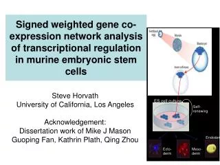
Answer: Overall, recent applications have convinced me that signed networks are preferable. • For example, signed networks were critical in a recent stem cell application • Michael J Mason, Kathrin Plath, Qing Zhou, et al (2009) Signed Gene Co-expression Networks for Analyzing Transcriptional Regulation in Murine Embryonic Stem Cells. BMC Genomics 2009, 10:327
Why construct a co-expression network based on the correlation coefficient ? • Intuitive • Measuring linear relationships avoids the pitfall of overfitting • Because many studies have limited numbers of arrays hard to estimate non-linear relationships • Works well in practice • Computationally fast • Leads to reproducible research
Relationship between Correlation and Mutual Information in case of an underlying linear relationship • Standardized mutual information represents soft-thresholding of correlation.
Why soft thresholding as opposed to hard thresholding? • Preserves the continuous information of the co-expression information • Results tend to be more robust with regard to different threshold choices But hard thresholding has its own advantages: In particular, graph theoretic algorithms from the computer science community can be applied to the resulting networks
Advantages of soft thresholding with the power function • Robustness: Network results are highly robust with respect to the choice of the power β (Zhang et al 2005) • Calibrating different networks becomes straightforward, which facilitates consensus module analysis • Math reason: Geometric Interpretation of Gene Co-Expression Network Analysis. PloS Computational Biology. 4(8): e1000117 • Module preservation statistics are particularly sensitive for measuring connectivity preservation in weighted networks
Questions:How should we choose the power beta or a hard threshold?Or more generally the parameters of an adjacency function?IDEA: use properties of the connectivity distribution
Generalized Connectivity • Gene connectivity = row sum of the adjacency matrix • For unweighted networks=number of direct neighbors • For weighted networks= sum of connection strengths to other nodes
Approximate scale free topology is a fundamental property of such networks (Barabasi et al) • It entails the presence of hub nodes that are connected to a large number of other nodes • Such networks are robust with respect to the random deletion of nodes but are sensitive to the targeted attack on hub nodes • It has been demonstrated that metabolic networks exhibit scale free topology at least approximately.
P(k) vs k in scale free networks P(k) • Scale Free Topology refers to the frequency distribution of the connectivity k • p(k)=proportion of nodes that have connectivity k • p(k)=Freq(discretize(k,nobins))
How to check Scale Free Topology? Idea: Log transformation p(k) and k and look at scatter plots Linear model fitting R^2 index can be used to quantify goodness of fit
Generalizing the notion of scale free topology Barabasi (1999) Csanyi-Szendroi (2004) Horvath, Dong (2005) Motivation of generalizations: using weak general assumptions, we have proven that gene co-expression networks satisfy these distributions approximately.
Checking Scale Free Topology in the Yeast Network • Black=Scale Free • Red=Exp. Truncated • Green=Log Log SFT
The scale free topology criterion for choosing the parameter values of an adjacency function. A) CONSIDER ONLY THOSE PARAMETER VALUES IN THE ADJACENCY FUNCTION THAT RESULT IN APPROXIMATE SCALE FREE TOPOLOGY, i.e. high scale free topology fitting index R^2 B) SELECT THE PARAMETERS THAT RESULT IN THE HIGHEST MEAN NUMBER OF CONNECTIONS • Criterion A is motivated by the finding that many networks (including gene co-expression networks, protein-protein interaction networks and cellular networks) have been found to exhibit a scale free topology • Criterion B leads to high power for detecting modules (clusters of genes) and hub genes.
Criterion A is measured by the linear model fitting index R2 Step AF (tau) Power AF (b) b= tau=
Trade-off between criterion A (R2) and criterion B (mean no. of connections) when varying thepower b criterion A: SFT model fit R^2 criterion B: mean connectivity
Trade-off between criterion A and B when varying tau Step Function: I(s>tau) criterion A criterion B
How to measure interconnectedness in a network?Answers: 1) adjacency matrix2)topological overlap matrix
Topological overlap matrix and corresponding dissimilarity (Ravasz et al 2002) • Generalization to weighted networks is straightforward since the formula is mathematically meaningful even if the adjacencies are real numbers in [0,1] (Zhang et al 2005 SAGMB) • Generalized topological overlap (Yip et al (2007) BMC Bioinformatics)
Set interpretation of the topological overlap matrix N1(i) denotes the set of 1-step (i.e. direct) neighbors of node i | | measures the cardinality Adding 1-a(i,j) to the denominator prevents it from becoming 0.
Generalizing the topological overlap matrix to 2 step neighborhoods etc • Simply replace the neighborhoods by 2 step neighborhoods in the following formula • www.genetics.ucla.edu/labs/horvath/GTOM Yip A et al (2007) BMC Bioinformatics 2007, 8:22
Module Definition • We often use average linkage hierarchical clustering coupled with the topological overlap dissimilarity measure. • Based on the resulting cluster tree, we define modules as branches • Modules are either labeled by integers (1,2,3…) or equivalently by colors (turquoise, blue, brown, etc)
Defining clusters from a hierarchical cluster tree: the Dynamic Tree Cut library for R. Langfelder P, Zhang B et al (2007) Bioinformatics 2008 24(5):719-720
Example: From: Ghazalpour et al (2006), PLoS Genetics Volume 2 Issue 8
Two types of branch cutting methods • Constant height (static) cut • cutreeStatic(dendro,cutHeight,minsize) • based on R function cutree • Adaptive (dynamic) cut • cutreeDynamic(dendro, ...) • Getting more information about the dynamic tree cut: • library(dynamicTreeCut) • help(cutreeDynamic) • More details: www.genetics.ucla.edu/labs/horvath/CoexpressionNetwork/BranchCutting/
Toy example of a cluster tree: Dendrogram (average linkage):
Constant height cut (a.k.a. static cut) Pick a height (in this case 6.5) and minimum size (in this case 3). Draw a line (red) at the chosen height. Look at all branches cut off by the line. Those that have at least 3 objects on them are modules. Label each module by a color to simplify identification. Objects outside of any module are labeled grey.
How do the clusters look like on the data? Yellow module appears to be missing its outer objects! Increase cut height?
Constant height cut at height = 15: Cut height is now too high: turquoise module swallowed its neighbor! Lesson: constant-height cut cannot identify tight and loose modules at the same time.
Summary Note that the dynamic hybrid method adaptively chooses the perfect height for each branch
A more complicated simulated example • Simulate 3 clusters, two of which are relatively close.
How will static cut perform? Static cut is not great since it either misses peripheral genes or it merges distinct clusters.
What about the dynamic cut? Looks better. Note the difference between Hybrid and Tree: Hybrid gets the outlying members more accurately.