Bayesian Statistics
This text delves into the fundamental differences between Bayesian and Frequentist paradigms in statistical analysis. The Frequentist approach defines probability as a long-run frequency and treats parameters as fixed, leading to hypothesis testing. In contrast, the Bayesian paradigm treats probability as subjective belief, viewing parameters as random variables. Using a clinical trial example of RU486 contraceptive, the analysis compares how each method evaluates effectiveness based on observed data. The text illustrates how different prior beliefs can significantly affect posterior probabilities and final conclusions.

Bayesian Statistics
E N D
Presentation Transcript
Bayesian Statistics Not in FPP
The Frequentist paradigm • Defines probability as a long-run frequency independent, identical trials • Looks at parameters (i.e., the true mean of the population, the true probability of heads) as fixed quantities • This paradigm leads one to specify the null and alternative hypotheses, collect data, calculate the significance probability under the assumption that the null is true, and draw conclusions based on these significance probabilities using size of the observed effects to guide decisions
The Bayesian paradigm • Defines probability as a subjective belief (which must be consistent with all of one’s other beliefs) • Looks at parameters (i.e., the true mean population, the true probability of heads) as random quantities because we can never know them with certainty • This paradigm leads one to specify plausible models to assign a prior probability to each model, to collect data, to calculate the probability of the data under each model, to use Baye’s theorm to calculate the posterior probability of each model, and to make inferences based on these posterior probabilities. The posterior probabilities enable one to make predictions about future observations and one uses one’s loss function to make decisions that minimize the probable loss
RU486 Example • The “morning after” contraceptive RU486 was tested in a clinical trial in Scotland. This discussion simplifies the design slightly. • Assum 800 women report to a clinic; they have each had sex within the last 72 hours. Half are randomly assigned to take RU486; half are randomly given the conventional theory (high dose of estrogen and synthetic progesterone). • Amone the RU486 group, none became pregnant. Among the conventional therapy group, there were 4 pregnancies. Does this show that RU 486 is more effective than conventional treatment? • Lets compare the frequentist and Bayesian approaches
RU486 Example • If the two therapies (R and C, for RU486 and conventional) are equally effective, then the probability that an observed pregnancy came from the R group is the proportion of women in the R group. (Here this would be 0.5). • Let p = Pr[an observed pregnancy came from group R]. • A frequentist wants to conduct a hypothesis test. Specifically Ho: p = 0.5 vs. Ha: p < 0.5 • If the evidence supports the alternative, then RU486 is more “effective” than the conventional procedure. • The data are 4 observations from a binomial, where p is the probability that a pregnancy is from group R • How do we calculate the significance probability?
RU486 Example • The significance probability is the chance of observing a result as or more extreme than the one in the sample, when the null hypothesis is true. • Our sample had no children from the R group, which is as supportive as we could have. So • p-value = Pr[0 successes in 4 tries | Ho true] = (1-0.5)4=0.0625 • Most frequentists would fail to reject, since 0.0625 > 0.05 • Suppose we had observed 1 pregnancy in the R group. What would the p-value be then?
RU486 Example • In the Bayesian analysis, we begin by listing the models we consider plausible. For example, suppose we thought we hade no information a priori about the probability that a child came from the R group. In that case all values of p between 0 and 1 would be equally likely. • Without calculus we cannot do that case, so let us approximate it by assuming that each of the following values for p 0.1, 0.2, 0.3, 0.3, 0.4, 0.5, 0.6, 0.7, 0.8, 0.9 is equally likely. So we consider 9 models, one for each value of the parameter p • If we picked one of the models say p=0.1, then that means the probability of a sample pregnancy coming from the R group is 0.1 and 0.9 that it comes from the C group. But we are not sure about the model
RU486 Example • So the most probable of the nine models has p=0.1. And the probability that p<0.5 is 0.427+0.267+0.156+0.084=0.934 • Note that in performing the Bayes calculation, • We were able to find the probability that p < 0.5, which we could not do in the frequentist framework. • In calculating this, we used only the data that we observed. Data that were more extreme than what we observed plays no role in the calculation or the logic. • Also note that the prior probability of p = 0.5 dropped from 1/9 = 0.111 to 0.041. This illustrates how our prior belief changes after seeing the data.
RU486 Example • Suppose a new person analyzes the same data. But their prior does not put equal weight on the 9 models; they put weight 0.52 on p=0.5 and equal weight on the others
RU486 Example • Compared to the first analyst, this one now believes that the probability that p=0.5 is 0.269, instead of 0.041. So the strong prior used by the second analyst has gotten a rather different result • But the probability that p=0.5 had dropped from 0.52 to 0.269, showing the evidence is running against the prior belief. • But in practice, what one really needs to know are predictive probabilities. For example, what is the probability that the next pregnancy comes from the RU486 group?
RU486 Example • To calculate the predictive probability for the next pregnancy, one finds the weighted average of the different p values, using the posterior probabilities as weights. • predictive probability = 0.1*0.326 + 0.2*0.204 +...+0.9*0.000= 0.281 • This is a very useful quantity, and on that cannot be calculated within the frequentist paradigm.