Download
1 / 33
360 likes | 520 Views
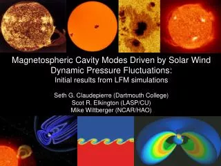
Magnetospheric Cavity Modes Driven by Solar Wind Dynamic Pressure Fluctuations: Initial results from LFM simulations Seth G. Claudepierre (Dartmouth College) Scot R. Elkington (LASP/CU) Mike Wiltberger (NCAR/HAO). Solar Wind Driving of ULF Pulsations. SW. SW.

E N D
Magnetospheric Cavity Modes Driven by Solar Wind Dynamic Pressure Fluctuations:Initial results from LFM simulations Seth G. Claudepierre (Dartmouth College) Scot R. Elkington (LASP/CU) Mike Wiltberger (NCAR/HAO)
Solar Wind Driving of ULF Pulsations SW SW ULF Waves Driven by Kelvin-Helmholtz Instability ULF Waves Driven by Solar Wind Dynamic Pressure Fluctuations * in this talk, ULF means frequencies less than 20 mHz or so
ULF Pulsations and the Radiation Belts ULF pulsation power is well-correlated with RB electron flux enhancements (e.g. Rostoker, 1998). Enegization and transport of RB electrons via ULF waves is mediated through a drift-resonant type interaction (Elkington, 1999; Hudson, 2000): An electron drifting in the equatorial plane with drift frequency ωd can be energized by a ULF wave with frequency ω = mωd where m is the azimuthal mode number of the wave. We need: frequency and azimuthal mode number spectrum of the ULF waves
ULF Pulsations and the Radiation Belts Physical characteristics of magnetospheric ULF waves known to be important for energization and transport of radiation belt electrons: A ULF wave with discrete spectral peaks at a particular ω and m determines the drift frequency of electrons that can be energized • The frequency spectrum at the discrete frequencies ω = mωdwhere ωd is the drift frequency of the interacting electron and m is • The azimuthal mode number of the interacting wave • The radial extent and • The azimuthal extent of the ULF waves determines the rate and location at which energization can occur. • The direction of propagation of the ULF waves
Solar Wind Driving of ULF Pulsations SW SW ULF Waves Driven by Kelvin-Helmholtz Instability ULF Waves Driven by Solar Wind Dynamic Pressure Fluctuations * in this talk, ULF means frequencies less than 20 mHz or so
ULF Waves Driven by KHI There is a strong correlation between ULF wave power in the magnetosphere and solar wind speed (e.g. Mathie and Mann, 2001). This observed correlation is often attributed to the Kelvin-Helmholtz instability at the magnetopause
ULF Waves Driven by KHI Claudepierre et al., JGR 2008, 113, A05218, doi:10.1029/2007JA012890. • KH waves generated at both the MP and the IEBL (near dawn and dusk flanks) over a wide range of Vsw (400-800 km/s); flow vortices at IEBL • KH wave amplitude depends on Vsw (increases as Vsw increases) • fε [5, 10] mHz (and wave frequency is dependent on Vsw) • λε [3, 6] Re and Vphaseε [150, 375] km/s (both dependent on Vsw) • azimuthal mode numbers, m≈ 15 (independent of Vsw) • coupled oscillation of both KH modes (and the entire dawn/dusk flank LLBL) • KH waves could resonant with radiation belt electrons in the 500 keV range
Solar Wind Driving of ULF Pulsations SW SW ULF Waves Driven by SW Pdyn Fluctuations ULF Waves Driven by KHI
ULF Waves Driven by SW Pdyn Fluctuations Several authors have noted that ULF variations In the solar wind number density can directly drive ULF pulsations in the magnetosphere (e.g. Kepko and Spence, 2003).
The LFM Global MHD Simulation Lyon-Fedder-Mobarry (LFM): single fluid, ideal MHD equations on 3D grid outer boundary condition: solar wind inner boundary condition: ionosphere computational grid: non-orthogonal, distorted spherical mesh (106x48x64) numerics: finite volume, 8th order spatial differencing, Adams-Bashforth time-stepping. caveats: no ring current, plasmasphere or radiation belts
Study Outline and Objectives Run the LFM with idealized solar wind input conditions to study the resultant magnetospheric ULF pulsations. In this study, we examine the magnetospheric response to upstream solar dynamic pressure fluctuations, both monochromatic and broadband. We examine 4 LFM simulations: three under monochromatic Pdyn driving (f = 5, 10, and 15 mHz) and one under quasi-broadband driving (f in 0 to 20 mHz) ULF Waves Driven by SW Pdyn Fluctuations SW SW input parameters: Vx = -600 km/s; Bz = -5 nT; Bx = By = 0; Vy = Vz = 0 …..and number density and sound speed….………
Monochromatic Pdyn Driving Monochromatic input density time series: - 3 monochromatic simulations (f = 5, 10, 15 mHz) - 20% oscillation amplitude on top of a background density (n0) of 5 particles/cc (i.e. C = 1). We also introduce the appropriate out of phase oscillation in the input sound speed so that the thermal pressure is constant in the input conditions ( Pth ~ n Cs2 ): = 40 km/s Remaining SW input parameters: Vx = -600 km/s; Bz = -5 nT; Bx = By = 0; Vy = Vz = 0
Broadband Pdyn Driving Broadband input density time series: The oscillation amplitude, D, is chosen so that the integrated power of input density time series in the broadband run is on the order of that in the monochromatic run. Hold input thermal pressure constant ( Pth ~ n Cs2 ): = 40 km/s Remaining SW input parameters: Vx = -600 km/s; Bz = -5 nT; Bx = By = 0; Vy = Vz = 0
Broadband Pdyn Driving Density, sound speed, thermal pressure and dynamic pressure time series in the input and upstream solar wind ( x = 20 Re ) in the broadband simulation Spectra of the above time series (green is input and blue is upstream).
Simulation Results: Waves Driven by SW Dynamic Pressure Fluctuations
Monochromatic Simulation Results: Ephi RIP in the Equatorial Plane 10 mHz Simulation 15 mHz Simulation RIP Over 9.5 to 10.5 mHz RIP Over 14.5 to 15.5 mHz
Monochromatic Simulation Results: Radial PSD Profiles Along 12 LT RIP Over 9.5 to 10.5 mHz RIP Over 14.5 to 15.5 mHz 15 mHz Simulation 10 mHz Simulation
Monochromatic Simulation Results Ephi and Bz Radial PSD Profiles Along 12 LT 10 mHz Run 15 mHz Run 5 mHz Run Ephi Bz Note: Bz has amplitude local maxima where Ephi has local minima (IB, MP, and BS)
Broadband Simulation Results Ephi PSD at (6.6, 0, 0) Ephi Radial PSD Along 12 LT Bz PSD The magnetosphere is clearly picking out two particular frequencies (~9 and 17 mHz) from the quasi-broadband upstream Pdyn fluctuations.
5 mHz Run 10 mHz Run 15 mHz Run BB Run Ephi RIP Bz RIP Simulation Results (mono. and broadband) Key Question: Why do the simulation results look so different under very similar driving (apart from the driving frequency)?
Magnetospheric Cavity Modes A simple cavity mode model can explain the simulation results: Magnetic and electric field oscillations modeled as standing waves between a cavity inner and outer boundary. Magnetospheric cavity modes are often invoked as drivers of FLR’s and have received substantial attention in theoretical/numerical models of the magnetosphere. Cavity modes have been studied numerically in simple geometries (e.g. box, cylindrical, and dipole magnetospheres) (in all 4 sims.)
n = 2 Cavity Mode in the 10 mHz Run 10 mHz Run 5 mHz Run • Ephi pulsation amplitude is larger in the 10 mHz run than in the 5 mHz run • 2) Ephi pulsation amplitude peak is near the magnetopause in the 5 mHz run but much more earthward in the 10 mHz run (~ 5 Re) Ephi RIP Bz RIP
n = 4 Cavity Mode in the 15 mHz Run 10 mHz Run 15 mHz Run • Ephi pulsation amplitude in the 15 mHz run has two peaks along the noon meridian (near 4 and 8 Re) • Bz pulsation amplitude increases strongly towards the simulation inner boundary in the 10 and 15 mHz runs, but not in the 5 mHz run. Ephi RIP Bz RIP
n = 2 and 4 Cavity Modes in the BB Run • There is a clear preferential frequency to the Ephi pulsation power (~9 mHz) • The 9 mHz wave power peaks near 5 Re. • There is a secondary preferential frequency in the Ephi pulsation power (~17 mHz) • The 17 mHz wave power has two radial peaks (near 4 and 8 Re). Ephi RIP Bz RIP
n = 6 Cavity Mode in the 25 mHz Run Results from a 25 mHz monochromatic simulation (where the n = 6 cavity mode should be excited):
No Odd Mode Number Cavity Modes? 5 mHz Run 10 mHz Run 15 mHz Run BB Run Ephi RIP Bz RIP
Time Out To Think Some natural questions to consider: • Q of the magnetospheric cavity? • What happens away from 12 LT? • Do these cavity modes couple energy into FLR’s?
Q of the Magnetospheric Cavity? 10 mHz Simulation w/ driving turned off
What Happens Away From 12 LT? 1800 LT As you move away from local noon, the cavity configuration changes, and thus the magnetospheric response frequency should change. 1640 LT 1440 LT 1200 LT MP BS Y X
What Happens Away From 12 LT? 1800 LT 1640 LT 1440 LT 1200 LT MP BS Y fmsphere = frequency of magnetospheric response X
FLR’s in the LFM Simulations? 10 mHz Simulation Er Amplitude and Phase (across afternoon sector peak at ~5 Re) Er RIP (integrated over 9.5 to 10.5 mHz)
Summary and Conclusions • ULF oscillations in the solar wind dynamic pressure can directly drive ULF pulsations in the magnetospheric electric and magnetic fields in the dayside (a la Kepko and Spence, 2003). • when the driving frequency matches the natural frequency of the magnetosphere, cavity modes can be energized • only even mode number cavity modes appear to be energized in the LFM simulations in this study