Download
1 / 31
310 likes | 349 Views
Get insights into MOSAIC's sensitivity to chirp, FROG's spectral autocorrelation, and GRENOUILLE's ultrashort pulse measurements. Learn how these techniques work and their applications in optics research.

E N D
Introduction to MOSAIC, SHG-FROG, and GRENOUILLE Ning Hsu 03/02/2016
Delay Modified Spectrum Auto Interferometric Correlation Interferometric Autocorrelation DC Intensity Autocorrelation I.F.T.{SH spectrum}
Delay Modified Spectrum Auto Interferometric Correlation x 2 MOSAIC Trace x 2 FFT-1 FFT 0 0 Delay Frequency Frequency 1) M. Sheik-Bahae, Opt. Lett.22, (1997) 2) T. Hirayama and M. Sheik-Bahae, Opt. Lett. 27, (2002)
MOSAIC in time Intensity Autocorrelation x 2 I.F.T.{SH spectrum}
Why MOSAIC? Interferometric Autocorrelation Not sensitive to pulse’s phase and shape?
Unchirped Chirped 1.0 1.0 0.8 0.8 0.6 0.6 0.4 0.4 0.2 0.2 0.0 0.0 -0.2 -0.2 -200 -100 0 100 200 -200 -100 0 100 200 Delay (fs) Delay (fs) 1.0 1.0 0.8 0.8 0.6 0.6 0.4 0.4 0.2 0.2 0.0 0.0 -200 -100 0 100 200 -200 -100 0 100 200 Delay (fs) Delay (fs) Less information leads to … more info? By eliminating the middle term, we get more sensitivity to chirp Interferometric Auto Correlation MOdified Spectrum Auto Interferometric Correlation The pulse is chirped, but how much?
Spectrum’s phase retrieving from MOSAIC Pass keep a and move on to b Second order coefficient a optimizing Does not pass change a and repeat delay delay delay Computed MOSAIC Trace Computed MOSAIC Trace Third order coefficient b optimizing Error function = difference between computed MOSAIC and experimental MOSACI (Using Nelder–Mead method to find the minimum) experimental MOSAIC Trace
Most people think of acoustic waves in terms of a musical score. It’s a plot of frequency vs. time, with information on top about the intensity. The musical score lives in the time-frequency domain.
Wigner distribution unchirped linearly chirped
Second-harmonic-generation FROG SHG FROG is simply a spectrally resolved autocorrelation. Pulse to be measured Beam splitter Camera E(t–t) SHG crystal Spec- trometer E(t) Esig(t,t)= E(t)E(t-t) Variable delay, t SHG FROG is the most sensitive version of FROG.
SHG FROG traces are symmetrical with respect to delay. Negatively chirped Unchirped Positively chirped Frequency Time Frequency Delay SHG FROG has an ambiguity in the direction of time, but it can be removed.
Generalized Projections Set of Esig(t,t) that satisfy the nonlinear-optical constraint: Esig(t,)E(t)E(t–) The Solution! Initial guess for Esig(t,) Set of Esig(t,t) that satisfy the data constraint: A projection maps the current guess for the waveform to the closest point in the constraint set. Convergence is guaranteed for convex sets, but generally occurs even with non-convex sets and in particular in FROG.
Ultrashort pulses measured using FROG FROG Traces Retrieved pulses Data courtesy of Profs. Bern Kohler and Kent Wilson, UCSD.
GRating-Eliminated No-nonsense Observationof Ultrafast Incident Laser Light E-fields(GRENOUILLE) FROG 2 key innovations: A single optic that replaces the entire delay line, and a thick SHG crystal that replaces both the thin crystal and spectrometer. GRENOUILLE C. Radzewicz, P. Wasylczyk, and J. S. Krasinski, Opt. Comm. 2000. P. O’Shea, M. Kimmel, X. Gu and R. Trebino, Optics Letters, 2001.
Pulse #1 Here, pulse #1 arrives earlier than pulse #2 x Here, the pulses arrive simultaneously Here, pulse #1 arrives later than pulse #2 Pulse #2 The Fresnel biprism Crossing beams at a large angle maps delay onto transverse position. Input pulse t=t(x) Fresnel biprism Even better, this design is amazingly compact and easy to use, and it never misaligns!
The thick crystal Very thin crystal creates broad SH spectrum in all directions. Standard autocorrelators and FROGs use such crystals. Thin crystal creates narrower SH spectrum in a given direction and so can’t be used for autocorrelators or FROGs. Thick crystal begins to separate colors. Thin SHG crystal Thick SHG crystal Very thick crystal acts like a spectrometer! Why not replace the spectrometer in FROG with a very thick crystal? Very thick crystal Suppose white light with a large divergence angle impinges on an SHG crystal. The SH generated depends on the angle. And the angular width of the SH beam created varies inversely with the crystal thickness. Very Thin SHG crystal
GRENOUILLE Beam Geometry Lens images position in crystal (i.e., delay, t) to horizontal position at camera Top view Imaging Lens Camera Cylindrical lens Fresnel Biprism Thick SHG Crystal FT Lens Lens maps angle (i.e., wavelength) to vertical position at camera Side view Yields a complete single-shot FROG. Uses the standard FROG algorithm. Never misaligns. Is more sensitive. Measures spatio-temporal distortions!
GVM is usually much greater than GVD GRENOUILLE requires a large GVM to spectrally resolve the pulse. But it requires a small GVD, or the pulse will spread. For all but near-single-cycle pulses (which are very broadband), GVM >> GVD, allowing us to satisfy both conditions simultaneously.
The GRENOUILLE operating range varies with wavelength. 80 3.5-mm BBO 70 60 Flat-phase pulse expands due to GVD GVM constraint (2.5 x device spectral resolution) 50 Bandwidth (nm) 40 30 20 10 0 500 600 700 800 900 1000 1100 1200 Wavelength (nm) Operation outside these limits is possible with corrections.
GRENOUILLE and crystal thickness A = ratio of pulse length or bandwidth and resolution limit The crystal must be thick and/or dispersive enough to frequency-resolve the pulse spectral structure (the GVM condition). Yet, the crystal must be thin and/or non-dispersive enough, or the pulse will spread in time (the GVD condition).
GRENOUILLE FROG Measured Retrieved Testing GRENOUILLE Compare a GRENOUILLE measurement of a pulse with a tried-and-true FROG measurement of the same pulse: Read more about GRENOUILLE in the cover story of OPN, June 2001 Retrieved pulse in the time and frequency domains
Tilted window Prism pair Input pulse Input pulse Spatially chirped output pulse Spatially chirped output pulse Angularly dispersed pulse with spatial chirp and pulse-front tilt Input pulse Prism Spatio-temporal distortions in pulses Prism pairs and simple tilted windows cause “spatial chirp.” Gratings and prisms cause both spatial chirp and “pulse-front tilt.” Angularly dispersed pulse with spatial chirp and pulse-front tilt Input pulse Grating
Signal pulse frequency 2w+dw Frequency 2wdw Tilt in the otherwise symmetrical SHG FROG trace indicates spatial chirp! Delay -t0 +t0 Fresnel biprism GRENOUILLE measures spatial chirp. SHG crystal Spatially chirped pulse -t0 +t0
GRENOUILLE accurately measures spatial chirp. Measurements confirm GRENOUILLE’s ability to measure spatial chirp. Positive spatial chirp Spatio-spectral plot slope (nm/mm) Negative spatial chirp
Zero relative delay is off to side of the crystal Zero relative delay is in the crystal center Frequency An off-center trace indicates the pulse front tilt! 0 Delay GRENOUILLE measures pulse-front tilt Fresnel biprism Tilted pulse front SHG crystal Untilted pulse front
GRENOUILLE accurately measures pulse-front tilt. Varying the incidence angle of the 4th prism in a pulse-compressor allows us to generate variable pulse-front tilt. Negative PFT Zero PFT Positive PFT
Disadvantages of GRENOUILLE Its low spectral resolution limits its use to pulse lengths between ~ 20 fs and ~ 1 ps. Like other single-shot techniques, it requires good spatial beam quality. Improvements on the horizon: Inclusion of GVD and GVM in FROG code to extend the range of operation to shorter and longer pulses.
Reference [1] D. A. Bender, Precision Optical Caracterization on NanometerLength and Femtosecond Time Scales. Ph.D dissertation, University of New Mexico, 2002 [2] J.-C. Diels and W. Rudolph, Ultrashort Laser Pulse Phenomena: Fundamentals, Techniques, and Applications on a Femtosecond Time scale. Academic Press, 1996.