CHAPTER
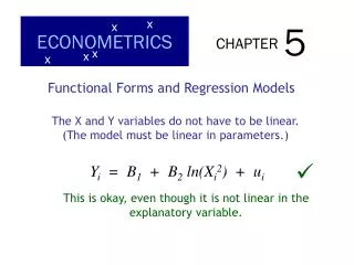
5. x. ECONOMETRICS. x. CHAPTER. x. x. x. Functional Forms and Regression Models. The X and Y variables do not have to be linear. (The model must be linear in parameters.). . Y i = B 1 + B 2 ln(X i 2 ) + u i. This is okay, even though it is not linear in the

CHAPTER
E N D
Presentation Transcript
5 x ECONOMETRICS x CHAPTER x x x Functional Forms and Regression Models The X and Y variables do not have to be linear. (The model must be linear in parameters.) Yi= B1 + B2 ln(Xi2) + ui This is okay, even though it is not linear in the explanatory variable.
Review of Logarithms Y= bX 10,000 = 104 logbY= X log1010,000 = 4 100 = e4.6051 loge100 = ln(100) = 4.6051 ln(AB) = ln(A) + ln(B) ln(Ak) = k ln(A) ln(1) = 0
The Log-Linear Model Yi= AXiB2 We ignore the error term, ui, for the time being. We can take the natural log of both sides: ln(Yi) = ln(AXiB2) ln(Yi) = ln(A) + B2ln(Xi) ln(Yi) = B1 + B2ln(Xi)
150 125 100 Quantity (100s) % ΔQD 75 % ΔP 50 25 20 40 60 80 100 120 Price ($) Price and Quantity Demand curve w/ constant slope Q = 150 – 1.25 P slope = -1.25 Price elasticity of demand = = slope x P/Q Elasticity = -1.25 x 40/100 = -0.5 Elasticity = -1.25 x 100/25 = -5.0
120 100 80 Quantity (100s) 60 40 20 20 40 60 80 100 120 Price ($) Constant price elasticity of demand Q = 64,000 P-2 slope = -128,000 P-3 Price elasticity of demand = slope x P/Q Elasticity = -0.25 x 80/10 = -2 Note: ln(Q) = ln(64,000) – 2 ln(P) ln(Q) = 11.07 - 2 ln(P) Elasticity = -2 x 40/40 = -2
Price and Quantity Linear (constant slope) model: If B2 = 2,150… $1 increase in price 2,150 more units. Qi= B1 + B2 Pi elasticity = B2 x Pi / Qi Log-linear (constant elasticity) model: If B2 = 0.45… 10% increase in price 4.5% increase in units ln(Qi) = B1 + B2ln(Pi) elasticity = B2
Multiple Log-Linear Models ln(Yi) = B1 + B2ln(X2i) + B3ln(X3i) + ui Cobb-Douglas Production Function Output= A (LaborB1)(CapitalB2) ln(Yi) = B1 + B2ln(Labori) + B3ln(Capitali) + ui
Constant returns to scale Double labor or capital, output increases but does not double. Double both labor and capital, output doubles.
Cobb-Douglas Production Function ln(Yi) = B1 + B2ln(Labori) + B3ln(Capitali) + ui Constant returns to scale: B2 + B3 = 1 Decreasing returns to scale: B2 + B3 < 1
The Semilog Model ln(Yi) = B1 + B2X2i + B3X3i + ui Log variable(s) only on one side of the equation. Most useful for variables that grow exponentially. Pop1 = 100 Pop2 = 100 x 1.04 = 104 Pop3 = 104 x 1.04 = 108.16 Pop4 = 1.0816 x 1.04 = 112.49
ln(Popi) = 4.63 + .0385 ti + ui A one year increase in time results in a 3.85% change in population

