Comprehensive Study of Motion Planning for Robotic Systems
320 likes | 350 Views
Explore translational and rotational motion planning for articulated robots, including Minkowski sums, free space computation, path computing, and connectivity graphs in this in-depth study.

Comprehensive Study of Motion Planning for Robotic Systems
E N D
Presentation Transcript
Motion Planning Shmuel Wimer Bar Ilan Univ., Eng. Faculty Technion, EE Faculty
Outline • Problem definition • Point robot • Work space and configuration space • Minkowski sums • Translational motion planning • Rotational motion planning
Articulated Robot Translation Motion goal start Types of Robots and Motions
Rotational Motion goal start Some robots can move in any direction (e.g., ants) Some robots cannot translate (e.g., cars) Given a robot, is there a free paths (no collisions) from start to goal? We’ll study translational and rotational motions
Reference Point Work Space and Configuration Space 2 Degrees of freedom 3 Degrees of freedom
Work space Configuration space
Divide into trapezoids. It takes O(nlogn) expected time. Remove trapezoids of obstacle in O(n) time. Free Space Computation
Building a Road Map Allocate node at center of vertical edges Allocate node at center of every trapezoid Connect center nodes to edge nodes Done in O(n) with doubly-connected edge list
Computing a Path Get from start to center of trapezoid in O(logn) time Get from goal to center of trapezoid in O(logn) time Connect center of trapezoids by BFS in O(n) time
Minkowski Sums Convert a problem with polygonal robot into point robot by modifying the obstacles in the configuration space to incorporate the geometry of the robot. robot obstacle
b 1 5 1 5 2 P b a a c 2 4 3 d 3 4 -R -R -R -R -R -R b b b b b b c a a a a a a c c c c c c d d d d d d d Construction of Minkowski Sum Edges of P and R are labeled counterclockwise
1 5 2 P a 4 3 4 5 2 b d -R b a c d 1 3 c
b 1 5 b a a a c 2 4 d 5 3 4 2 b d c d 1 3 c
Minkowski sum for ladder at 0º rotation. Blockage exists. Rotation – Moving a Ladder
Minkowski sum for ladder at 30º rotation. Blockage exists. Minkowski sum for ladder at 60º rotation. Blockage changed.
Front view. θ varies from 0º to 75º. Bottom view Conversion to 3D Motion Problem Ladder’s reference point can move in the 3D space!
Obstacles Minkowski sums 2 1 C 9 A ∞ 10 8 3 B 7 6 5 Cell decomposition R Ladder 4 Cell Decomposition
A Cell is the collection of all free points labeled with the same front/back edge label pairs. • A: (3,2); B: (3,8); C: (1,9) • Cell decomposition has discontinuities when ladder is oriented similar to an edge. • There are finite number of ladder rotation where cell decomposition is changing. • New cells can appear and old ones may disappear.
C disappeared 2 1 9 ∞ A 10 8 3 B 7 6 5 R 4 Ladder is rotated
C: (1,9) (1,∞) (10,∞) (5,∞) (3,∞) G0º B: (3,8) (1,8) A: (3,2) In Connectivity GraphGθ nodes are cells of decomposition and edges are connecting nodes corresponding to adjacent cells in free area (a kind of dual graph).
(1,∞) (10,∞) (5,∞) (1,8) (3,∞) B: (3,8) A: (3,2) (4,∞) (7,8) Critical Orientations correspond to slants of edges.
Connectivity Graph G is constructed by stacking the connectivity graphs Gθ corresponding to the critical orientations. Vertices of two distinct Gθ are connected iff they are labeled with the same edge pair. Starting from G0, Gθ are added in increasing order of θ, thus creating a layered 3D graph. A paths from start to goal if exists can be found by a BFS algorithm.