Download
1 / 14
240 likes | 721 Views
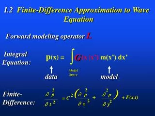
. 2. 2. . p. p. 2. +. + F(x,t). = C. 2. t. 2. p. 2. 2. y. x. p (x) = (x |x’) m(x’) dx’. G. Integral Equation:. ò. model. data. Model Space. Finite- Difference:. I.2 Finite-Difference Approximation to Wave Equation.

E N D
2 2 p p 2 + + F(x,t) = C 2 t 2 p 2 2 y x p(x) = (x |x’) m(x’) dx’ G Integral Equation: ò model data Model Space Finite- Difference: I.2 Finite-Difference Approximation to Wave Equation Forward modeling operator L
Pressure 2 = C + + F(x,t) 2 2 2 p p p 2 2 2 y x t Source Term 2-D Acoustic Wave Equation p(x,0) Initial Conditions: Boundary Conditions: ; p (x,0): t=0, all x t p(x,t) on boundaries of model, all t
FD Approximation to 2-D Acoustic Wave Equation t p ij i t F ij j p (x,y,t) x F (x,y,t) t y
FD Approximation to 2-D Acoustic Wave Equation t t+1 - p p ij ij i j t+ t p(x,y,t) t x t t + O(t) z 1st-order Forward FD Approx.
FD Approximation to 2-D Acoustic Wave Equation t-1 t - p p ij ij t j t- t+ t t p(x,y,t) t t + O(t) z 1st-order backward FD Approx.
FD Approximation to 2-D Acoustic Wave Equation Backward FD 2 p(x,y,t) 2 t t t-1 t Forward FD - p p ij ij t t t-1 t+1 t p p p 2nd-order central FD Approx. - 2 + ij ij ij = t 2 p(x,y,t) = t ij =
FD Approximation to 2-D Acoustic Wave Equation Forward FD Backward FD 2 p(x,y,t) 2 t t t x x x t t p p p - 2 + i-1j i+1j ij = x 2 2nd-order central FD Approx. p(x,y,t) = t
FD Approximation to 2-D Acoustic Wave Equation Forward FD Backward FD 2 p(x,y,t) 2 y y t t t p p p - 2 + ij-1 ij+1 ij = y 2 2nd-order FD stencil p(x,y,t) = y
FD Approximation to 2-D Acoustic Wave Equation 2 2 c t Future Past t-1 t+1 t t t t t t t p p p p p p p - 2 + p - 2 p - 2 + + ij ij ij i+1j ij-1 ij ij+1 ij + = i-1j y 2 x 2 t + F ij Rearrange so that future P’s are on LHS and past and present P’s are on RHS
FD Approximation to 2-D Acoustic Wave Equation Future Past & Present t t t t t t p p p t+1 p t-1 p - 2 p t - 2 + p 2 p + 2 p c t - 2 = i+1j ij-1 + ij ij+1 ij + ij i-1j ij ij y 2 2 x t + F ij Given: Panels at t, t-1 Find: Panel at t+1
FD Approximation to 2-D Acoustic Wave Equation t-1 t Past & Present t+1 Given: Panels at t, t-1 Find: Panel at t+1 Future t t t t t t p p p t+1 p p t-1 - 2 p t + p - 2 2 p + 2 p c t - 2 = i+1j ij-1 + ij ij+1 ij + ij i-1j ij ij y 2 2 x t + F ij
Fortran Code FD Approx. to 2-D Acoustic Wave Equation fort=1:nt for i=1:nx for j=1:ny t t t t t t p p p t+1 p t-1 p - 2 p t - 2 + p 2 p + 2 p c t - 2 = i+1j ij-1 + ij ij+1 ij + ij i-1j ij ij y 2 2 x t + F end end end
MATLAB Code FD Approx. to 2-D Acoustic Wave Equation a = (c*dt/dx)^2; fort=1:nt f = force(:,:,t); dfuture = dpres - 2* dpast + a*del(dpres); dfuture = dfuture + f; dpast=dpresent; dpresent=dfuture; end
MATLAB Exercise: Forward Modeling 1. Retrieve MATLAB program fd.m, and execute it for a simple point source at depth. Observe reflections off the free surface. Why does the polarity change sign for free-surface reflections? A). Why does the polarity change sign for free-surface reflections? B). Stability is guaranteed if dt/dx*c < .7. Change dt so stability is violated. What happens to snapshots. C). Dispersion condition is that dx is less than .1*wavelength. Change dx so stability is ok but dispersion condition is violated. What is result? D). Why do reflections emanate from side-boundaries?