Face Detection

1. Face Detection CSE 576

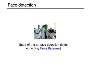
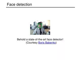
2. Face detection State-of-the-art face detection demo (Courtesy Boris Babenko)

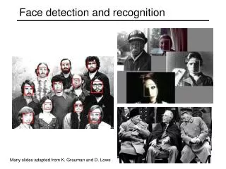
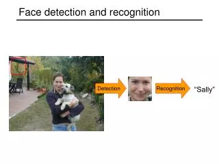
3. Face detection and recognition Detection Recognition “Sally”

4. Face detection • Where are the faces?

5. Face Detection • What kind of features? • What kind of classifiers?

6. Image Features +1 -1 “Rectangle filters” Value = ∑ (pixels in white area) – ∑ (pixels in black area)

7. Feature extraction “Rectangular” filters • Feature output is difference between adjacent regions • Efficiently computable with integral image: any sum can be computed in constant time • Avoid scaling images scale features directly for same cost Viola & Jones, CVPR 2001 K. Grauman, B. Leibe

8. Sums of rectangular regions How do we compute the sum of the pixels in the red box? After some pre-computation, this can be done in constant time for any box. This “trick” is commonly used for computing Haar wavelets (a fundemental building block of many object recognition approaches.)

9. Sums of rectangular regions The trick is to compute an “integral image.” Every pixel is the sum of its neighbors to the upper left. Sequentially compute using:

10. Sums of rectangular regions Solution is found using: A + D – B - C What if the position of the box lies between pixels?

11. Large library of filters • Considering all possible filter parameters: position, scale, and type: • 180,000+ possible features associated with each 24 x 24 window Use AdaBoost both to select the informative features and to form the classifier Viola & Jones, CVPR 2001 K. Grauman, B. Leibe

12. Feature selection • For a 24x24 detection region, the number of possible rectangle features is ~160,000! • At test time, it is impractical to evaluate the entire feature set • Can we create a good classifier using just a small subset of all possible features? • How to select such a subset?

13. AdaBoost for feature+classifier selection Want to select the single rectangle feature and threshold that best separates positive (faces) and negative (non-faces) training examples, in terms of weighted error. Resulting weak classifier: For next round, reweight the examples according to errors, choose another filter/threshold combo. … Outputs of a possible rectangle feature on faces and non-faces. Viola & Jones, CVPR 2001 K. Grauman, B. Leibe

14. AdaBoost: Intuition Consider a 2-d feature space with positive and negative examples. Each weak classifier splits the training examples with at least 50% accuracy. Examples misclassified by a previous weak learner are given more emphasis at future rounds. K. Grauman, B. Leibe Figure adapted from Freund and Schapire

15. AdaBoost: Intuition K. Grauman, B. Leibe

16. AdaBoost: Intuition Final classifier is combination of the weak classifiers K. Grauman, B. Leibe

17. Final classifier is combination of the weak ones, weighted according to error they had. K. Grauman, B. Leibe

18. AdaBoost Algorithm Start with uniform weights on training examples {x1,…xn} For T rounds Find the best threshold and polarity for each feature, and return error. Re-weight the examples: Incorrectly classified -> more weight Correctly classified -> less weight

19. Recall • Classification • NN • Naïve Bayes • Logistic Regression • Boosting • Face Detection • Simple Features • Integral Images • Boosting

20. Measuring classification performance • Confusion matrix • Accuracy • (TP+TN)/(TP+TN+FP+FN) • True Positive Rate=Recall • TP/(TP+FN) • False Positive Rate • FP/(FP+TN) • Precision • TP/(TP+FP) • F1 Score • 2*Recall*Precision/(Recall+Precision)

21. Boosting for face detection • First two features selected by boosting:This feature combination can yield 100% detection rate and 50% false positive rate

22. Boosting for face detection • A 200-feature classifier can yield 95% detection rate and a false positive rate of 1 in 14084 Is this good enough? Receiver operating characteristic (ROC) curve

23. T T T T FACE IMAGE SUB-WINDOW Classifier 2 Classifier 3 Classifier 1 F F F NON-FACE NON-FACE NON-FACE Attentional cascade • We start with simple classifiers which reject many of the negative sub-windows while detecting almost all positive sub-windows • Positive response from the first classifier triggers the evaluation of a second (more complex) classifier, and so on • A negative outcome at any point leads to the immediate rejection of the sub-window

24. % False Pos 0 50 vs false neg determined by 0 100 % Detection Attentional cascade Receiver operating characteristic • Chain classifiers that are progressively more complex and have lower false positive rates: T T T T FACE IMAGE SUB-WINDOW Classifier 2 Classifier 3 Classifier 1 F F F NON-FACE NON-FACE NON-FACE

25. Attentional cascade • The detection rate and the false positive rate of the cascade are found by multiplying the respective rates of the individual stages • A detection rate of 0.9 and a false positive rate on the order of 10-6 can be achieved by a 10-stage cascade if each stage has a detection rate of 0.99 (0.9910 ≈ 0.9) and a false positive rate of about 0.30 (0.310 ≈ 6×10-6) T T T T FACE IMAGE SUB-WINDOW Classifier 2 Classifier 3 Classifier 1 F F F NON-FACE NON-FACE NON-FACE

26. Training the cascade • Set target detection and false positive rates for each stage • Keep adding features to the current stage until its target rates have been met • Need to lower AdaBoost threshold to maximize detection (as opposed to minimizing total classification error) • Test on a validation set • If the overall false positive rate is not low enough, then add another stage • Use false positives from current stage as the negative training examples for the next stage

27. Viola-Jones Face Detector: Summary Train cascade of classifiers with AdaBoost Apply to each subwindow Faces New image Selected features, thresholds, and weights Non-faces Train with 5K positives, 350M negatives Real-time detector using 38 layer cascade 6061 features in final layer [Implementation available in OpenCV: http://www.intel.com/technology/computing/opencv/] K. Grauman, B. Leibe

28. The implemented system • Training Data • 5000 faces • All frontal, rescaled to 24x24 pixels • 300 million non-faces • 9500 non-face images • Faces are normalized • Scale, translation • Many variations • Across individuals • Illumination • Pose

29. System performance • Training time: “weeks” on 466 MHz Sun workstation • 38 layers, total of 6061 features • Average of 10 features evaluated per window on test set • “On a 700 Mhz Pentium III processor, the face detector can process a 384 by 288 pixel image in about .067 seconds” • 15 Hz • 15 times faster than previous detector of comparable accuracy (Rowley et al., 1998)

30. Non-maximal suppression (NMS) Many detections above threshold.

31. Non-maximal suppression (NMS)

32. Is this good? Similar accuracy, but 10x faster

33. Viola-Jones Face Detector: Results K. Grauman, B. Leibe

34. Viola-Jones Face Detector: Results K. Grauman, B. Leibe

35. Viola-Jones Face Detector: Results K. Grauman, B. Leibe

36. Detecting profile faces? Detecting profile faces requires training separate detector with profile examples. K. Grauman, B. Leibe

37. Viola-Jones Face Detector: Results K. Grauman, B. Leibe Paul Viola, ICCV tutorial

38. Summary: Viola/Jones detector • Rectangle features • Integral images for fast computation • Boosting for feature selection • Attentional cascade for fast rejection of negative windows