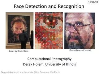
Face detection and recognition
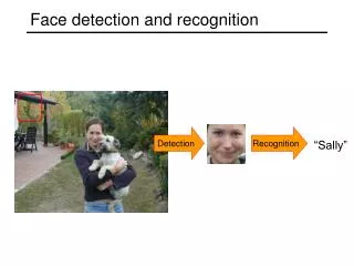
Face detection and recognition. Detection. Recognition. “Sally”. Face detection & recognition. Viola & Jones detector Available in open CV Face recognition Eigenfaces for face recognition Metric learning identification . Face detection. Many slides adapted from P. Viola.

Face detection and recognition
E N D
Presentation Transcript
Face detection and recognition Detection Recognition “Sally”
Face detection & recognition • Viola & Jones detector • Available in open CV • Face recognition • Eigenfaces for face recognition • Metric learning identification
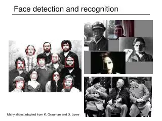
Face detection Many slides adapted from P. Viola
Consumer application: iPhoto 2009 http://www.apple.com/ilife/iphoto/
Challenges of face detection • Sliding window detector must evaluate tens of thousands of location/scale combinations • Faces are rare: 0–10 per image • For computational efficiency, we should try to spend as little time as possible on the non-face windows • A megapixel image has ~106 pixels and a comparable number of candidate face locations • To avoid having a false positive in every image image, our false positive rate has to be less than 10-6
The Viola/Jones Face Detector • A seminal approach to real-time object detection • Training is slow, but detection is very fast • Key ideas • Integral images for fast feature evaluation • Boosting for feature selection • Attentional cascade for fast rejection of non-face windows P. Viola and M. Jones. Rapid object detection using a boosted cascade of simple features. CVPR 2001. P. Viola and M. Jones. Robust real-time face detection. IJCV 57(2), 2004.
Image Features “Rectangle filters” Value = ∑ (pixels in white area) – ∑ (pixels in black area)
Fast computation with integral images • The integral image computes a value at each pixel (x,y) that is the sum of the pixel values above and to the left of (x,y), inclusive • This can quickly be computed in one pass through the image (x,y)
Computing the integral image • Cumulative row sum: s(x, y) = s(x–1, y) + i(x, y) • Integral image: ii(x, y) = ii(x, y−1) + s(x, y) ii(x, y-1) s(x-1, y) i(x, y)
Computing sum within a rectangle • Let A,B,C,D be the values of the integral image at the corners of a rectangle • Then the sum of original image values within the rectangle can be computed as: sum = A – B – C + D • Only 3 additions are required for any size of rectangle! D B A C
Feature selection • For a 24x24 detection region, the number of possible rectangle features is ~160,000!
Feature selection • For a 24x24 detection region, the number of possible rectangle features is ~160,000! • At test time, it is impractical to evaluate the entire feature set • Can we create a good classifier using just a small subset of all possible features? • How to select such a subset?
Boosting • Boosting is a classification scheme that works by combining weak learners into a more accurate ensemble classifier • Training consists of multiple boosting rounds • During each boosting round, we select a weak learner that does well on examples that were hard for the previous weak learners • “Hardness” is captured by weights attached to training examples Y. Freund and R. Schapire, A short introduction to boosting, Journal of Japanese Society for Artificial Intelligence, 14(5):771-780, September, 1999.
Training procedure • Initially, weight each training example equally • In each boosting round: • Find the weak learner that achieves the lowest weighted training error • Raise the weights of training examples misclassified by current weak learner • Compute final classifier as linear combination of all weak learners (weight of each learner is directly proportional to its accuracy) • Exact formulas for re-weighting and combining weak learners depend on the particular boosting scheme (e.g., AdaBoost)
Boosting vs. SVM • Advantages of boosting • Integrates classifier training with feature selection • Flexibility in the choice of weak learners, boosting scheme • Testing is very fast • Disadvantages • Needs many training examples • Training is slow • Often doesn’t work as well as SVM (especially for many-class problems)
Boosting for face detection • Define weak learners based on rectangle features value of rectangle feature parity threshold window
Boosting for face detection • Define weak learners based on rectangle features • For each round of boosting: • Evaluate each rectangle filter on each example • Select best filter/threshold combination based on weighted training error • Reweight examples
Boosting for face detection • First two features selected by boosting:This feature combination can yield 100% detection rate and 50% false positive rate
T T T T FACE IMAGE SUB-WINDOW Classifier 2 Classifier 3 Classifier 1 F F F NON-FACE NON-FACE NON-FACE Attentional cascade • We start with simple classifiers which reject many of the negative sub-windows while detecting almost all positive sub-windows • Positive response from the first classifier triggers the evaluation of a second (more complex) classifier, and so on • A negative outcome at any point leads to the immediate rejection of the sub-window
% False Pos 0 50 vs false neg determined by 0 100 % Detection Attentional cascade • Chain classifiers that are progressively more complex and have lower false positive rates: Receiver operating characteristic T T T T FACE IMAGE SUB-WINDOW Classifier 2 Classifier 3 Classifier 1 F F F NON-FACE NON-FACE NON-FACE
Attentional cascade • The detection rate and the false positive rate of the cascade are found by multiplying the respective rates of the individual stages • A detection rate of 0.9 and a false positive rate on the order of 10-6 can be achieved by a 10-stage cascade if each stage has a detection rate of 0.99 (0.9910 ≈ 0.9) and a false positive rate of about 0.30 (0.310 ≈ 6×10⁻⁶) T T T T FACE IMAGE SUB-WINDOW Classifier 2 Classifier 3 Classifier 1 F F F NON-FACE NON-FACE NON-FACE
Training the cascade • Set target detection and false positive rates for each stage • Keep adding features to the current stage until its target rates have been met • Need to lower AdaBoost threshold to maximize detection (as opposed to minimizing total classification error) • Test on a validation set • If the overall false positive rate is not low enough, then add another stage • Use false positives from current stage as the negative training examples for the next stage
The implemented system • Training Data • 5000 faces • All frontal, rescaled to 24x24 pixels • 300 million non-faces • 9500 non-face images • Faces are normalized • Scale, translation • Many variations • Across individuals • Illumination • Pose
System performance • Training time: “weeks” on 466 MHz Sun workstation • 38 layers, total of 6061 features • Average of 10 features evaluated per window on test set • “On a 700 Mhz Pentium III processor, the face detector can process a 384 by 288 pixel image in about .067 seconds” • 15 Hz
Summary: Viola/Jones detector • Rectangle features • Integral images for fast computation • Boosting for feature selection • Attentional cascade for fast rejection of negative windows
Face detection & recognition • Viola & Jones detector • Available in open CV • Face recognition • Eigenfaces for face recognition • Metric learning identification
The space of all face images • When viewed as vectors of pixel values, face images are extremely high-dimensional • 100x100 image = 10,000 dimensions • However, relatively few 10,000-dimensional vectors correspond to valid face images • We want to effectively model the subspace of face images
The space of all face images • We want to construct a low-dimensional linear subspace that best explains the variation in the set of face images
Principal Component Analysis • Given: N data points x1, … ,xNin Rd • We want to find a new set of features that are linear combinations of original ones:u(xi) = uT(xi – µ)(µ: mean of data points) • What unit vector u in Rd captures the most variance of the data?
Principal Component Analysis • Direction that maximizes the variance of the projected data: N Projection of data point N Covariance matrix of data The direction that maximizes the variance is the eigenvector associated with the largest eigenvalue of Σ
Principal component analysis • The direction that captures the maximum covariance of the data is the eigenvector corresponding to the largest eigenvalue of the data covariance matrix • Furthermore, the top k orthogonal directions that capture the most variance of the data are the k eigenvectors corresponding to the k largest eigenvalues
Eigenfaces: Key idea • Assume that most face images lie on a low-dimensional subspace determined by the first k (k<d) directions of maximum variance • Use PCA to determine the vectors or “eigenfaces” u1,…uk that span that subspace • Represent all face images in the dataset as linear combinations of eigenfaces M. Turk and A. Pentland, Face Recognition using Eigenfaces, CVPR 1991
Eigenfaces example • Training images • x1,…,xN
Eigenfaces example Top eigenvectors: u1,…uk Mean: μ
Eigenfaces example • Face x in “face space” coordinates: • Reconstruction: = = + ^ x = µ + w1u1+w2u2+w3u3+w4u4+ …
Recognition with eigenfaces • Process labeled training images: • Find mean µ and covariance matrix Σ • Find k principal components (eigenvectors of Σ) u1,…uk • Project each training image xi onto subspace spanned by principal components:(wi1,…,wik) = (u1T(xi – µ), … , ukT(xi – µ)) • Given novel image x: • Project onto subspace:(w1,…,wk) = (u1T(x– µ), … , ukT(x– µ)) • Classify as closest training face in k-dimensional subspace ^ M. Turk and A. Pentland, Face Recognition using Eigenfaces, CVPR 1991
Limitations • Global appearance method: not robust to misalignment, background variation
Limitations • PCA assumes that the data has a Gaussian distribution (mean µ, covariance matrix Σ) The shape of this dataset is not well described by its principal components
Limitations • The direction of maximum variance is not always good for classification
Face detection & recognition • Viola & Jones detector • Available in open CV • Face recognition • Eigenfaces for face recognition • Metric learning for face identification
Learning metrics for face identification • Are these two faces of the same person? • Challenges: • pose, scale, lighting, ... • expression, occlusion, hairstyle, ... • generalization to people not seen during training M. Guillaumin, J. Verbeek and C. Schmid. Metric learning for face identification. ICCV’09.
Metric Learning • Most common form of learned metrics are Mahalanobis • M is a positive definite matrix • Generalization of Euclidean metric (setting M=I) • Corresponds to Euclidean metric after linear transformation of the data
Logistic Discriminant Metric Learning • Classify pairs of faces based on distance between descriptors • Use sigmoid to map distance to class probability
Logistic Discriminant Metric Learning • Mahanalobis distance linear in elements of M • Linear logistic discriminant model • Distance is linear in elements of M • Learn maximum likelihood M and b • Can use low-rank M =LTL to avoid overfitting • Loses convexity of cost function, effective in practice
Feature extraction process • Detection of 9 facial features[Everingham et al. 2006] • using both appearance and relative position • using the constellation mode • leads to some pose invariance • Each facial features described using SIFT descriptors
Feature extraction process • Detection of 9 facial features • Each facial features described using SIFT descriptors at 3 scales • Concatenate 3x9 SIFTs into a vector of dimensionality 3456