VERY LONG BASELINE INTERFEROMETRY
VERY LONG BASELINE INTERFEROMETRY. Craig Walker. WHAT IS VLBI?. Radio interferometry with unlimited baselines High resolution – milliarcsecond (mas) or better Baselines up to an Earth diameter for ground based VLBI Can extend to space (HALCA) Sources must have high brightness temperature

VERY LONG BASELINE INTERFEROMETRY
E N D
Presentation Transcript
VERY LONG BASELINE INTERFEROMETRY Craig Walker
WHAT IS VLBI? • Radio interferometry with unlimited baselines • High resolution – milliarcsecond (mas) or better • Baselines up to an Earth diameter for ground based VLBI • Can extend to space (HALCA) • Sources must have high brightness temperature • Traditionally uses no IF or LO link between antennas • Data recorded on tape or disk then shipped to correlator • Atomic clocks for time and frequency– usually hydrogen masers • Correlation occurs days to years after observing • Real time over fiber is an area of active development • Can use antennas built for other reasons • Not fundamentally different from linked interferometry Mark5 recorder Maser Ninth Synthesis Imaging Summer School, 15-22 June 2004
THE QUEST FOR RESOLUTION Atmosphere gives 1" limit without corrections which are easiest in radio Jupiter and Io as seen from Earth 1 arcmin 1 arcsec 0.05 arcsec 0.001 arcsec Simulated with Galileo photo
GLOBAL VLBI STATIONS Geodesy stations. Some astronomy stations missing, especially in Europe. Ninth Synthesis Imaging Summer School, 15-22 June 2004
The VLBA Ten 25m Antennas, 20 Station Correlator 327 MHz - 86 GHz National Radio Astronomy Observatory A Facility of the National Science Foundation
M87 Inner Jet EXAMPLE 1JET FORMATION:BASE OF M87 JET VLA Images • 43 GHz Global VLBI • Junor, Biretta, & Livio Nature, 401, 891 • Shows hints of jet collimation region Resolution 0.000330.00012 Black Hole / Jet Model VLBI Image
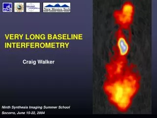
EXAMPLE 2: JET DYNAMICS: THE SS433 MOVIE • Two hour snapshot almost every day for 40 days on VLBA at 1.7 GHz • Mioduszewski, Rupen, Taylor, and Walker Ninth Synthesis Imaging Summer School, 15-22 June 2004
EXAMPLE 3MOTIONS OF SGRA* Measures rotation of the Milky Way Galaxy 0.00590.4 / yr Reid et al. 1999, Ap. J. 524, 816 Ninth Synthesis Imaging Summer School, 15-22 June 2004
10 cm Baseline Length 1984-1999 Baseline transverse 10 cm EXAMPLE 4GEODESY and ASTROMETRY Germany to Massachusetts • Fundamental reference frames • International Celestial Reference Frame (ICRF) • International Terrestrial Reference Frame (ITRF) • Earth rotation and orientation relative to inertial reference frame of distant quasars • Tectonic plate motions measured directly • Earth orientation data used in studies of Earth’s core and Earth/atmosphere interaction • General relativity tests • Solar bending significant over whole sky GSFC Jan 2000 Ninth Synthesis Imaging Summer School, 15-22 June 2004
VLBI and CONNECTED INTERFEROMETRYDIFFERENCES VLBI is not fundamentally different from connected interferometry Differences are a matter of degree. Separate clocks –Cause phase variations Independent atmospheres (ionosphere and troposphere) Phase fluctuations not much worse than VLA A array Gradients are worse – affected by total, not differential atmosphere Ionospheric calibration useful – dual band data or GPS global models Calibrators poor Compact sources are variable – Calibrate using Tsys and gains All bright sources are at least somewhat resolved – need to image There are no simple polarization position angle calibrators Geometric model errors cause phase gradients Source positions, station locations, and the Earth orientation are difficult to determine to a small fraction of a wavelength Ninth Synthesis Imaging Summer School, 15-22 June 2004
VLBI and CONNECTED INTERFEROMETRYDIFFERENCES (CONTINUED) Phase gradients in time and frequency need calibration – fringe fit VLBI is not sensitive to thermal sources 106 K brightness temperature limit This limits the variety of science that can be done Hard to match resolution with other bands like optical An HST pixel is a typical VLBI field of view Even extragalactic sources change structure on finite time scales VLBI is a movie camera Networkshave inhomogeneous antennas – hard to calibrate Much lower sensitivity to RFI Primary beam is not usually an issue for VLBI Ninth Synthesis Imaging Summer School, 15-22 June 2004
VLBA Station Electronics At antenna: Select RCP and LCP Add calibration signals Amplify Mix to IF (500-1000 MHz) In building: Distribute to baseband converters (8) Mix to baseband Filter (0.062 - 16 MHz) Sample (1 or 2 bit) Format for tape (32 track) Record Also keep time and stable frequency Other systems conceptually similar VLBA STATION ELECTRONICS Ninth Synthesis Imaging Summer School, 15-22 June 2004
VLBI CORRELATOR • Read tapes or disks • Synchronize data • Apply delay model • Includes phase model • Correct for known Doppler shifts • Mainly from Earth rotation • This is the total fringe rate and is related to the rate of change of delay • Generate cross and auto correlation power spectra • FX: FFT or filter, then cross multiply (VLBA, Nobeyama, ATA, GMRT) • XF: Cross multiply lags. FFT later (JIVE, Haystack, VLA, EVLA, ALMA …) • Accumulate and write data to archive • Some corrections may be required in postprocessing • Data normalization and scaling (Varies by correlator) • Corrections for clipper offsets (ACCOR in AIPS) JIVE Correlator Ninth Synthesis Imaging Summer School, 15-22 June 2004
THE DELAY MODEL For 8000 km baseline 1 mas = 3.9 cm = 130 ps Adapted from Sovers, Fanselow, and Jacobs Reviews of Modern Physics, Oct 1998 Ninth Synthesis Imaging Summer School, 15-22 June 2004
VLBI Data Reduction Ninth Synthesis Imaging Summer School, 15-22 June 2004
VLBI Amplitude Calibration • Scij = Correlated flux density on baseline i - j • = Measured correlation coefficient • A = Correlator specific scaling factor • s= System efficiency including digitization losses • Ts = System temperature • Includes receiver, spillover, atmosphere, blockage • K = Gain in degrees K per Jansky • Includes gain curve • e- = Absorption in atmosphere plus blockage • Note Ts/K = SEFD (System Equivalent Flux Density) Ninth Synthesis Imaging Summer School, 15-22 June 2004
CALIBRATION WITH Tsys Example shows removal of effect of increased Ts due to rain and low elevation Ninth Synthesis Imaging Summer School, 15-22 June 2004
Atmospheric opacity Correcting for absorption by the atmosphere Can estimate using Ts – Tr – Tspill Example from single-dish VLBA pointing data GAIN CURVES AND OPACITY CORRECTION VLBA gain curves Caused by gravity induced distortions of the antenna as a function of elevation 4cm 2cm 20cm 1cm 50cm 7mm
PULSE CAL SYSTEM • Tones generated by injecting pulse once per microsecond • Use to correct for instrumental phase shifts pcal tones A Data Aligned using Pulse Cal Pulse cal monitor data A No PCAL at VLA. Shows unaligned phases Long track at non-VLBA station
IONOSPHERIC DELAY • Delay scales with 1/2 • Ionosphere dominates errors at low frequencies • Can correct with dual band observations (S/X) • GPS based ionosphere models help (AIPS task TECOR) Maximum Likely Ionospheric Contributions Ionosphere map from iono.jpl.nasa.gov Delays from an S/X Geodesy Observation -20 Delay (ns) 20 8.4 GHz2.3 GHz Time (Days)
A (Jy) (deg) A (Jy) (deg) Raw Data - No Edits EDITING • Flags from on-line system will remove most bad data. Examples: • Antenna off source • Subreflector out of position • Synthesizers not locked • Final flagging done by examining data • Flag by antenna • Most problems are antenna based • Poor weather • Bad playback • RFI (May need to flag by channel) • First point in scan sometimes bad A (Jy) (deg) A (Jy) (deg) Raw Data - Edited Ninth Synthesis Imaging Summer School, 15-22 June 2004
BANDPASS CALIBRATION Covered in detail in next lecture • Based on bandpass calibration source • Effectively a self-cal on a per-channel basis • Needed for spectral line calibration • May help continuum calibration by reducing closure errors • Affected by high total fringe rates • Fringe rate shifts spectrum relative to filters • Bandpass spectra must be shifted to align filters when applied • Will lose edge channels in process of correcting for this. Before After Ninth Synthesis Imaging Summer School, 15-22 June 2004
AMPLITUDE CHECK SOURCE Typical calibrator visibility function after a priori calibration Calibrator is resolved Will need to image One antenna low Use calibrator to fix Shows why flux scale (gain normalization) should only be set by a subset of antennas Resolved – a model or image will be needed Poorly calibrated antenna Ninth Synthesis Imaging Summer School, 15-22 June 2004
FRINGE FITTING • Raw correlator output has phase slopes in time and frequency • Slope in time is “fringe rate” • Usually from imperfect troposphere or ionosphere model • Slope in frequency is “delay” • A phase slope because • Fluctuations worse at low frequency because of ionosphere • Troposphere affects all frequencies equally ("nondispersive") • Fringe fit is self calibration with first derivatives in time and frequency Ninth Synthesis Imaging Summer School, 15-22 June 2004
FRINGE FITTING: WHY • For Astronomy: • Remove clock offsets and align baseband channels (“manual pcal”) • Done with 1 or a few scans on a strong source • Could use bandpass calibration if smearing corrections were available • Fit calibrator to track most variations (optional) • Fit target source if strong (optional) • Used to allow averaging in frequency and time • Allows higher SNR self calibration (longer solution, more bandwidth) • Allows corrections for smearing from previous averaging • Fringe fitting weak sources rarely needed any more • For geodesy: • Fitted delays are the primary “observable” • Slopes are fitted over wide spanned frequency range • “Bandwidth Synthesis” • Correlator model is added to get “total delay”, independent of models Ninth Synthesis Imaging Summer School, 15-22 June 2004
FRINGE FITTING: HOW • Two step process (usually) • 2D FFT to get estimated rates and delays to reference antenna • Required for start model for least squares • Can restrict window to avoid high sigma noise points • Can use just baselines to reference antenna or can stack 2 and even 3 baseline combinations • Least squares fit to phases starting at FFT estimate • Baseline fringe fit • Not affected by poor source model • Used for geodesy. Noise more accountable. • Global fringe fit • One phase, rate, and delay per antenna • Best SNR because all data used • Improved by good source model • Best for imaging and phase referencing Ninth Synthesis Imaging Summer School, 15-22 June 2004
SELF CALIBRATION IMAGING • Iterative procedure to solve for both image and gains: • Use best available image to solve for gains (can start with point) • Use gains to derive improved image • Should converge quickly for simple sources • Many iterations (~50-100) may be needed for complex sources • May need to vary some imaging parameters between iterations • Should reach near thermal noise in most cases • Can image even if calibration is poor or nonexistent • Possible because there are N antenna gains and N(N-1)/2 baselines • Need at least 3 antennas for phase gains, 4 for amplitude gains • Works better with many antennas • Does not preserve absolute position or flux density scale • Gain normalization usually makes this problem minor • Is required for highest dynamic ranges on all interferometers Ninth Synthesis Imaging Summer School, 15-22 June 2004
Example Self Cal Imaging Sequence • Start with phase only selfcal • Add amplitude cal when progress slows (#3 here) • Vary parameters between iterations • Taper, robustness, uvrange etc • Try to reach thermal noise • Should get close Ninth Synthesis Imaging Summer School, 15-22 June 2004
PHASE REFERENCING • Calibration using phase calibrator outside target source field • Nodding calibrator (move antennas) • In-beam calibrator (separate correlation pass) • Multiple calibrators for most accurate results – get gradients • Similar to VLA calibration except: • Geometric and atmospheric models worse • Affected by totals between antennas, not just differentials • Model errors usually dominate over fluctuations • Errors scale with total error times source-target separation in radians • Need to calibrate often (5 minute or faster cycle) • Need calibrator close to target (< 5 deg) • Biggest problems: • Wet troposphere at high frequency • Ionosphere at low frequencies (20 cm is as bad as 1cm) • Use for weak sources and for position measurements • Increases sensitivity by 1 to 2 orders of magnitude • Used by about 30-50% of VLBA observations
EXAMPLE OF REFERENCED PHASES • 6 min cycle - 3 on each source • Phases of one source self-calibrated (near zero) • Other source shifted by same amount Ninth Synthesis Imaging Summer School, 15-22 June 2004
Phase Referencing Example • With no phase calibration, source is not detected (no surprise) • With reference calibration, source is detected, but structure is distorted (target-calibrator separation is probably not small) • Self-calibration of this strong source shows real structure No Phase Calibration Reference Calibration Self-calibration Ninth Synthesis Imaging Summer School, 15-22 June 2004
SCHEDULING • PI provides the detailed observation sequence • The schedule should include: • Fringe finders (strong sources - at least 2 scans – helps operations) • Amplitude check source (strong, compact source) • If target is weak, include a delay/rate calibrator • If target very weak, fast switch to a phase calibrator • For spectral line observations, include bandpass calibrator • For polarization observations, calibrate instrumental terms • Get good Parallactic angle coverage on polarized source or • Observe an unpolarized source • Absolute polarization position angle calibrator (Get angle from VLA) • Leave occasional gaps for tape readback tests (2 min) • For non-VLBA observations, manage tapes • Tape passes and tape changes • With Mark5, only worry about total data volume Ninth Synthesis Imaging Summer School, 15-22 June 2004
THE END Ninth Synthesis Imaging Summer School, 15-22 June 2004