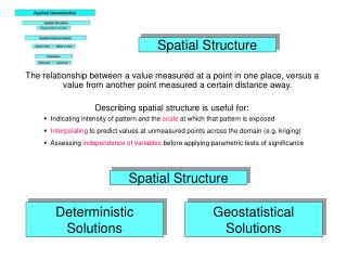
Spatial Structure
Spatial Structure. The relationship between a value measured at a point in one place, versus a value from another point measured a certain distance away. Describing spatial structure is useful for:. Indicating intensity of pattern and the scale at which that pattern is exposed

Spatial Structure
E N D
Presentation Transcript
Spatial Structure The relationship between a value measured at a point in one place, versus a value from another point measured a certain distance away. Describing spatial structure is useful for: • Indicating intensity of pattern and the scale at which that pattern is exposed • Interpolating to predict values at unmeasured points across the domain (e.g. kriging) • Assessing independence of variables before applying parametric tests of significance Spatial Structure Deterministic Solutions Geostatistical Solutions
Deterministic Solutions Predicted Model Measured First Order Polynomial Interpolation Second Order (third, fourth, etc.) Polynomial Interpolation Local Polynomial Interpolation Radial Basis Function (Spline) Interpolation
Geostatistical Solutions Semivariance The geostatistical measure that describes the rate of change of the regionalized variable is known as the semivariance. Semivariance is used for descriptive analysis where the spatial structure of the data is investigated using the semivariogram and for predictive applications where the semivariogram is fitted to a theoretical model, parameterized, and used to predict the regionalized variable at other non-measured points (kriging). Where : j is a point at distance d from i ndis the number of points in that distance class (i.e., the sum of the weights wij for that distance class) wij is an indicator function set to 1 if the pair of points is within the distance class.
Spatial Pattern is an outcome of the synthesis of dynamic processes operating at various spatial and temporal scales Given: Therefore: Structure at any given time is but one realization of several potential outcomes Assuming: All processes are Stationary (homogeneous) Properties are independent of absolute location and direction in space Where: That is: Observations are independent which := they are homoscedastic and form a known distribution Therefore: Stationarity is a property of the process NOT the data, allowing spatial inferences And: Furthermore: Stationarity is scale dependent Inference (spatial statistics) apply over regions of assumed stationarity Thus: Geostatistical Solutions - Semivariance
100 100 5 4 3 2 1 0 Given: ?? 105 Where: Is spatial dependent of an intrinsic stationary process 105 Find: 115 We assume: 0 1 2 3 4 5 Where: is known, and IDW (inverse distance weighting) depends only on distance Kriging depends upon semivariogram which considers spatial relationship and distance Is the weight at (i) We constrain the prediction such that: That says: The difference between the predicted and the observed should be small OR: minimize the statistical expectations of:
value @ i – value @ j Empirical Semivariogram ½ the difference squared between pairs Semivariogram 1st, recall that Euclidean distance is; Distance between paired points 2nd, Empirical semivariance := NOTE: In large dataset this can become unmanageable. Solution: Binning pairs at the similar distances such as (1,5) and (1,3) 3rd, Bin ranges of distances; and find …. • Average Distance between all pairs in each bin • Average Semivariance of all paired observations in each bin
5th, Knowing , construct the matrix (Gamma) for the sample location, 13.5 4th, Plot the Semivariogram and fit a model (ie.: least-squares regression passing through zero) Empirical Fitted Semivariance = slope*distance Semivariance = 13.5 * h Average Semivariance in each bin Average Distance in bin h For example, pair (1,5) and (3,4), the lag distance is calculated using the distance between the two locations; the semivariogram value is found by multiplying the slope (13.5) time the distance. = 30.19 *
Recalling from the Empirical Semivariogram: Semivariance = slope * distance Semivariance = 13.5 * h 5th, Without resorting to matrix algebra; the next step constructs the matrix of all model semivariance for all pairs … such that: Gamma Matrix is the model’s semivariance for all sampled pairs Where: , or Lambda vector contains weights assign to the measured values surrounding the location to be predicted Where: Where: Gamma vector is the prediction from all location Such that: Which yields: 6th, This means that in our example, to predict the value at location (1,4) the vector is such that: Slope*distance=slope*h=13.5*1
5 4 3 2 1 0 0 1 2 3 4 5 7th, This mean that in our example, to predict the value at location (1,4) with the the matrix and the vector, we can: step 5, step 6 102.6218 Solve: 100 100 105 Such That: 105 115 Kriging Predictor
For predictions, the empirical semivariogram is converted to a theoretic one by fitting a statistical model (curve) to describe its range, sill, & nugget. There are four common models used to fit semivariograms: Assumes no sill or range Linear: Exponential: Spherical: Where: c0 = nugget b = regression slope a = range c0+ c = sill Gaussian:
A semivariogram is a plot of the structure function that, like autocorrelation, describes the relationship between measurements taken some distance apart. Semivariograms define the range or distance over which spatial dependence exists. • The nugget is the semivariance at a distance 0.0, (the y –intercept) • The sill is the value at which the semivariogram levels off (its asymptotic value) • The range is the distance at which the semivariogram levels off (the spatial extent of structure in the data)
Stationarity • Autocorrelation assumes stationarity, meaning that the spatial • structure of the variable is consistent over the entire domain of the dataset. • The stationarity of interest is second-order (weak) stationarity, requiring that: • the mean is constant over the region • variance is constant and finite; and • covariance depends only on between-sample spacing • In many cases this is not true because of larger trends in the data • In these cases, the data are often detrended before analysis. • One way to detrend data is to fit a regression to the trend, and use only the residuals for autocorrelation analysis
Anistotropy Autocorrelation also assumes isotropy, meaning that the spatial structure of the variable is consistent in all directions. Often this is not the case, and the variable exhibits anisotropy, meaning that there is a direction-dependent trend in the data. If a variable exhibits different ranges in different directions, then there is a geometric anisotropy. For example, in a dune deposit, larger range in the wind direction compared to the range perpendicular to the wind direction.
Variogram Modeling Suggestions • Check for enough number of pairs at each lag distance (from 30 to 50). • Removal of outliers • Truncate at half the maximum lag distance to ensure enough pairs • Use a larger lag tolerance to get more pairs and a smoother variogram • Start with an omnidirectional variogram before trying directional variograms • Use other variogram measures to take into account lag means and variances (e.g., inverted covariance, correlogram, or relative variograms) • Use transforms of the data for skewed distributions (e.g. logarithmic transforms). • Use the mean absolute difference or median absolute difference to derive the range