Download
1 / 26
420 likes | 984 Views
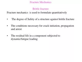
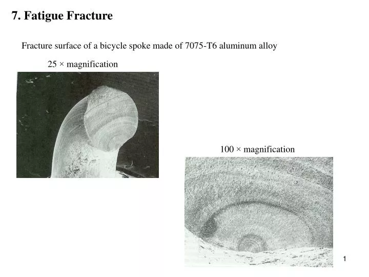
7. Fatigue Fracture. Fracture surface of a bicycle spoke made of 7075-T6 aluminum alloy. 25 × magnification. 100 × magnification. Introduction:.

E N D
7. Fatigue Fracture Fracture surface of a bicycle spoke made of 7075-T6 aluminum alloy 25 × magnification 100 × magnification
Introduction: • When metals are subjected to fluctuating load, the failure occurs at a stress level much lower than the fracture stress corresponding to a monotonic tension load. • With the development of the railway (<1900) much attention was given to the understanding of the fatigue failure phenomenon. • August Wöhler (1819-1914), director of Imperial Railways in Germany from 1847 to 1889 - First investigator to address fatigue tests on railway axles and small-scale specimens. - Provided plots of the failure stress as a function of the number of cycles to failure Useful for the total life prediction of a part subjected to constant amplitude cyclic loading: Wöhler S-N diagrams The Wöhler approach was next extended to other areas : bridges, ships, machinery equipment … • It is still used to assess fatigue failure of modern structures (e.g. aircraft components) subjected to repeated loading.
High-cycle fatigue when material failure occurs under a large number of cycles ( > 100000 ) : Strains and stresses are within the elastic range. Laboratory tests for constructing the S-N diagram in given environmental conditions (inertial, thermal, pressure stresses …). • Low-cycle fatigue failure (100-100000 cycles) : Magnitude of fluctuating stresses does not remain in the elastic range. Significant plastic straining may occur throughout the structure, especially at stress concentrators. Cannot be characterized by S-N curves. • To prevent fatigue failure of a structural part, in general ones needs : (1) All loading events that a component will experience + number of times that each one occurs. (2) Empirical equation relating the fatigue crack growth da/dN with the crack tip SIF DK . (3) Material fracture toughness. (4) Some estimate of the initial flaw size. Calculation of the remaining life cycles
Cyclic or Fluctuating load : Sa 1) Constant amplitude cyclic loading : Amplitude and mean stress stay constant. S Five stress parameters that can defined the loading characteristics: Maximum stress : Minimum stress : Alternatively, Cyclic stress amplitude : Mean stress: Stress Ratio: Any two of the above quantities are sufficient to completely define cyclic loading.
Typical constant amplitude loading cycles Stress Stress Stress Stress Stress Time Time Time Time Time
Stress Time The maximum and minimum cyclic stresses are equal and For the same range, R=-1 is considered to be a less damaging cyclic load when evaluating the fatigue life of a structure. Example: Rotating-bending test using 4 point-bending to apply a constant moment to a rotating cylindrical specimen.
Stress Stress Time Time The minimum stress equals zero. Example: Pressurization and depressurization cycle of a pressurized tank Both maximum and minimum stresses are positive. Example: Preloaded bolt subjected to cyclic tensile stresses such that the minimum and maximum fatigue stresses are positive
Stress Time Both maximum and minimum stresses are negative. Example: Plate with a hole that undergone a sleeve cold expansion = mandrelizing process that creates a massive zone of compressive residual stress field fatigue tensile load applied Mandrelized hole under fluctuating load with smax =0. The minimum stress is negative. For the same stress range, R>0 is considered to be the most damaging cyclic load when evaluating the fatigue life of a structure. R= 1 : static loading
2) Random loading : Time Stress Typical cyclic loads in real structures almost random in nature and vary in magnitude . Complex and may contain any combination of the above cyclic cases. Example: Loading environment of a aircraft or space structure during is lifetime. 3) Fatigue spectrum : All loading events and the number of times that each event occurs are reported . Each event may be a function of several variables. The irregular load sequence Sum of cycles Ni with associated Si and
Load environments for a space component: • Prelaunch cycles (acceptance , proof testing, …) • Transportation cycles prior to flight • Flight cycles • On-orbit cycles due to on-orbit activities • Thermal cycles Different methods to establish a fatigue spectrum from time history data : Rain flow method Fatigue and Fracture Mechanics of high risk parts, Bahram Farahmand (1997)
Constant amplitude axial fatigue tests : For the determination of the fatigue life of a metallic part: - predominantly elastic stresses - high number of cycling Laboratory fatigue tests with typical types of specimens: Recommended by the ASTM E-466 Diameter : D : 0.25- 2.5 cm Area Wt : 0.07- 2.5 cm2 2<W/t <6 L : 5.3 cm, R : 10.16 cm Designed such failure occurs in the middle region.
The S-N diagram • Principle of similitude: The life of a structural part is the same as the life of a test specimen if both undergo the same nominal stress s Service loading of a bridge exposed to a fluctuating load: Laboratory fatigue specimen subjected to the same nominal stress s
S-N curve definition: Plot of stress amplitude S versus the number of cycles to failure Nf maximun stress smax Nf : dependant variable Endurance limit or fatigue limit
Log S Log Nf • Other representations: smax or S most widely used Semi-logarithmic plotting : and Log N Log smax or Log S and Logarithmic plotting : Log N Typical S-N curve for ferrous alloys Endurance limit • Endurance limit: - is not a constant and generally varies with R - depends on the types of load: lower in uniaxial loading than in reverse bending - Affected by the degree of surface finish, heat treatment, stress concentration, corrosive environment A well-defined fatigue limit is not always existing.
S-N diagram for 4340 alloy steel: Endurance limit of 43.3 ksi (1 ksi= 6.895 MPa) with R = -1
S-N diagram for 2024-T4 aluminum alloy Endurance limit not well defined.
Linear cumulative damage when Total damage = result of several fluctuating stresses at different levels S-N diagram useful to determine the number of cycles of failure with a given constant amplitude applied cyclic stress . The contributing damage caused by each load environment should be evaluated. Fatigue damage at a given stress level = number of cycles applied at that stress level Nfi = total number of cycles to fail the part at the same stress level Palmgren-Miner rule (1945) Total failure: Based on the linear summation rule for damage (see eq. 2.12)
Application of the Palmgren-Miner rule: (ksi) (ksi) Decreasing R Decreasing R A component of space structure made of allow steel : - is subjected to fluctuating loads with different stress magnitudes: See launch and on-orbit fatigue spectrum given table 1 - has the following S-N curve: R = 0, -0.1, -0.3 , -0.5 , -1 1 ksi = 6.895 MPa Including a safe-life factor of 4, will the part survive the load environment (R = -1) ?
Sum all The number of cycles to failure, Nfi associated to the loading step i is given by: First step: Idem for the other loading steps (launch + on-orbit + thermal) Multiply the expression by the safe-life factor of 4 Check if the summation <1
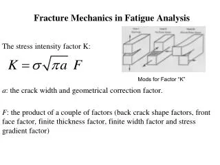
Stress Intensity factor range and crack growth rate Fatigue crack propagation investigated using the fracture mechanics concepts: Time-dependent mode I loading The SIF factor is now time dependant : We define a maximum / minimum SIF
Problem : Time to grow the crack up to a certain length or until fracture of the part ? if Small scaling yielding SIF characterizes the crack tip field. Similitude principle: same behavior for cracks with the same FIC. then The crack propagation law can be expressed by : Average crack speed Fracture thoughness No crack growth below : threshold value of SIF
Difficult to derive theoretically ! empirically obtained in order to fit experimental data Number of cycles to grow the crack from a0 to a:
Typical crack growth data and the curve fit for 2024-T861 aluminum alloy
5-8% 1-2% 85-90% versus is linear Typical fatigue crack growth behavior Observed for a large class of materials Region 1: slow crack advance Region 2: intermediate, higher speeds Region 3: fast crack growth, very short in time approximate % of life spent Similar to the endurance limit : threshold value of SIF Region II can be described by such a power law: Earliest relation of Paris and Erdogan (1960), widely used. A and n empirical parameters (see table 7.1)
Noting we have, assuming that Integration of Paris & Erdogan law: Therefore by integration,
More general, valid in all regions, takes into account the ratio R, the fracture toughness KIC , the limit Failure occurs at the crack length ac when Solving for ac and reporting in the previous equations: One obtains Nc : number of cycles to fracture Others models than the model of Paris & Erdogan are reported: Forman-Newman- de Koning (FNK) law (1992): C, n, p, q are empirically constants f is a function that models the crack closure effect. widely used in aerospace structures for life estimation of high risk fracture critical parts.