Download
1 / 41
410 likes | 520 Views
TB Cluster Models, Time Scales and Relations to HIV. Carlos Castillo-Chavez. Department of Biological Statistics and Computational Biology Department of Theoretical and Applied Mechanics Cornell University, Ithaca, New York, 14853. Outline.

E N D
TB Cluster Models, Time Scales and Relations to HIV Carlos Castillo-Chavez Department of Biological Statistics and Computational Biology Department of Theoretical and Applied Mechanics Cornell University, Ithaca, New York, 14853 MTBI Cornell University
Outline • A non-autonomous model that incorporates the impact of HIV on TB dynamics. • Model to test CDC’s TB control goals. • Casual versus close contacts and their impact on TB. • Time scales and singular perturbation approaches in the study of the dynamics of TB. MTBI Cornell University
TB in the US(1953-1999) MTBI Cornell University
Reemergence of TB • New York City and San Francisco had • recent outbreaks. • Cost of control the outbreak in NYC alone • was estimated to be about 1 billion. • Observed national TB case rate increase. • TB reemergence became an international • issue. • CDC sets control goal in 1989. MTBI Cornell University
Basic Model Framework • N=S+E+I+T, Total population • F(N): Birth and immigration rate • B(N,S,I): Transmission rate (incidence) • B`(N,S,I): Transmission rate (incidence) MTBI Cornell University
Model Equations MTBI Cornell University
CDC Short-Term Goal: 3.5 cases per 100,000 by 2000. Has CDC met this goal? CDC Long-term Goal: One case per million by 2010. Is it feasible? TB control in the U.S. MTBI Cornell University
Model Construction Since d has been approximately equal to zero over the past 50 years in the US, we only consider Hence, N can be computed independently of TB. MTBI Cornell University
Non-autonomous model (permanent latent class of TB introduced) MTBI Cornell University
Effect of HIV MTBI Cornell University
Upper Bound and Lower Bound For Epidemic Threshold If R<1, L1(t), L2(t) and I(t) approach zero; If R>1, L1(t), L2(t) and I(t) all have lower positive boundary; If (t) and d(t) are time-independent, R and R are Equal to R0 . MTBI Cornell University
Parameter estimation and simulation setup MTBI Cornell University
Parameter estimation and simulation setup N(t) is from census data and population projection MTBI Cornell University
RESULTS MTBI Cornell University
CONCLUSIONS MTBI Cornell University
CONCLUSIONS MTBI Cornell University
CDC’s Goal Delayed • Impact of HIV. • Lower curve does not include HIV impact; • Upper curve represents the case rate when HIV is included; • Both are the same before 1983. Dots represent real data. MTBI Cornell University
Regression approach A Markov chain model supports the same result MTBI Cornell University
Cluster Models • Incorporates contact type (close vs. casual) and focus on the impact of close and prolonged contacts. • Generalized households become the basic epidemiological unit rather than individuals. • Use natural epidemiological time-scales in model development and analysis. MTBI Cornell University
Close and Casual contacts Close and prolonged contacts are likely to be responsible for the generation of most new cases of secondary TB infections. “A high school teacher who also worked at library infected the students in her classroom but not those who came to the library.” Casual contacts also lead to new cases of active TB. WHO gave a warning in 1999 regarding air travel. It announced that flights of more than 8 hours pose a risk for TB transmission. MTBI Cornell University
Transmission Diagram MTBI Cornell University
Key Features • Basic epidemiological unit: cluster (generalized household) • Movement of kE2 to I class brings nkE2 to N1population, where by assumptions nkE2(S2 /N2) go to S1 and nkE2(E2/N2) go to E1 • Conversely, recovery of I infectious bring nI back to N2 population, where nI (S1 /N1)= S1 go to S2 and nI (E1 /N1)= E1 go to E2 MTBI Cornell University
Basic Cluster Model MTBI Cornell University
Basic Reproductive Number where is the expected number of infections produced by one infectious individual within his/her cluster. denotes the fraction who survives the latency period and become active cases. MTBI Cornell University
Diagram of Extended Cluster Model MTBI Cornell University
(n) Both close casual contacts are included in the extended model. The risk of infection per susceptible, , is assumed to be a nonlinear function of the average cluster size n. The constant p measures the average proportion of the time that an “individual spends in a cluster. MTBI Cornell University
R0 Depends on n in a non-linear fashion MTBI Cornell University
Role of Cluster Size E(n) denotes the ratio of within cluster to between cluster transmission. E(n) increases and reaches its maximum value at The cluster size n* is defined as optimal as it maximizes the relative impact of within to between cluster transmission. MTBI Cornell University
Full system Hoppensteadt’s Theorem(1973) Reduced system where x Rm, y Rn and is a positive real parameter near zero (small parameter). Five conditions must be satisfied (not listed here) to apply the theorem. In addition, it is shown that if the reduced system has a globally asymptotically stable equilibrium then the full system has a g.a.s. equilibrium whenever 0< <<1. MTBI Cornell University
Two time Scales • Latent period is long and roughly has the same order of magnitude as that associated with the life span of the host. • Average infectious period is about six months (wherever there is treatment, is even shorter). MTBI Cornell University
Rescaling Time is measured in average infectious periods (fast time scale), that is, = k t. The state variables are rescaled as follow: Where / is the asymptotic carrying capacity. MTBI Cornell University
Rescaled Model MTBI Cornell University
Rescaled Model MTBI Cornell University
Dynamics on Slow Manifold Solving for the quasi-steady states y1, y2 and y3in terms of x1 and x2 gives Substituting these expressions into the equations for x1 and x2 lead to the equations of motion on the slow manifold. MTBI Cornell University
Slow Manifold Dynamics Where is the number of secondary infections produced by one infectious individual in a population where everyone is susceptible MTBI Cornell University
Theorem If Rc0 1,the disease-free equilibrium (1,0) is globally asymptotically stable. While if Rc0 > 1, (1,0) is unstable and the endemic equilibrium is globally asymptotically stable. This theorem characterizes the dynamics on the slow manifold MTBI Cornell University
Dynamics for Full System Theorem: For the full system, disease-free equilibrium is globally asymptotically stable whenever R0c <1; while R0c >1 there exists a unique endemic equilibrium which is globally asymptotically stable. Proof approach: Construct Lyapunov function for the case R0c <1; for the case R0c >1, we use Hoppensteadt’s Theorem. A similar result can be found in Z. Feng’s 1994, Ph.D. dissertation. MTBI Cornell University
1 Bifurcation Diagram Global bifurcation diagram when 0<<<1 where denotes the ratio between rate of progression to active TB and the average life-span of the host (approximately). MTBI Cornell University
Numerical Simulations MTBI Cornell University
Conclusions from cluster models • TB has slow dynamics but the change of • epidemiological units makes it possible to identify • non-traditional fast and slow dynamics. • Quasi steady assumptions (adiabatic elimination of • parameter) are valid (Hoppensteadt’s theorem). • The impact of close and casual contacts can be study • using this approach as long as progression rates • from the latently to the actively-infected stages are • significantly different. MTBI Cornell University
Conclusions from cluster models • Singular perturbation theory can be used to study the global asymptotic dynamics. • Optimal cluster size highlights the relative impact of close versus casual contacts and suggests alternative mechanisms of control. • The analysis of the system for the case where the small parameter is not small has not been carried out. Simulations suggest a wider range. MTBI Cornell University