Download
1 / 15
150 likes | 263 Views
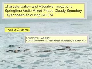
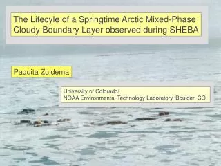
The Lifecyle of a Springtime Arctic Mixed-Phase Cloudy Boundary Layer observed during SHEBA. Paquita Zuidema. University of Colorado/ NOAA Environmental Technology Laboratory, Boulder, CO. Surface Heat Budget of the Arctic. SHEBA. Early May ~ 76N, 165 W. WHY ?.

E N D
The Lifecyle of a Springtime Arctic Mixed-Phase Cloudy Boundary Layer observed during SHEBA Paquita Zuidema University of Colorado/ NOAA Environmental Technology Laboratory, Boulder, CO
Surface Heat Budget of the Arctic SHEBA
Early May ~ 76N, 165 W
WHY ? • GCMs indicate Arctic highly responsive to increasing greenhouse gases (e.g. IPCC) • Clouds strongly influence the arctic surface and atmosphere, primarily through radiative interactions • Factors controlling arctic cloudiness not well known • Springtime conditions of particular interest
What I’ve done: • Picked a multi-day time period containing aircraft data as well as the ship-board data • Used the aircraft data to help strengthen the shipboard assessment of the cloud properties, so that a 9-day cloud characterization could be done w/ confidence • Used the cloud characterization to assess the cloud’s radiative impact and elucidate the cloud lifecycle Why so challenging ?? both ice and liquid phases are present (cloud T ~ -15C)
Surface-based Instrumentation: May 1-8 time series 8 dBZ -20 -45 -5 6 35 GHzcloudradar ice cloud properties km 4 2 depolarization lidar-determined liquid cloud base Microwave radiometer-derived liquid water paths 100 g/m^2 2 3 4 5 6 7 8 1 day day 4X daily soundings.Near-surface T ~ -20 C, inversion T ~-10 C 1 4 lidar cloud base 8 z -30C -10C
Details of the cloud characterization can be found athttp://www.etl.noaa.gov/~pzuidema publication now in press with J. Atmos. Sci. Cloud radar reflectivity -50 0 dBZ Brad Baker & Paul Lawson - aircraft data and analysis knowledge Yong Han - new and improved liquid water paths Janet Intrieri - depolarization lidar data Jeff Key - Streamer radiative transfer code Sergey Matrosov - cloud radar retrieval of ice cloud properties Robert Stone - sunphotometer-derived aerosol optical depths Matthew Shupe & Taneil Uttal - well-organized, web-accessible datasets -50 2 Height (km) 1 Temperature inversion Aircraft path Lidar cloud base UTC 24:00 22:00 23:00 time
Main results from cloud characterization • Liquid cloud phase adiabatically-distributed • Radar ice microphysical retrievals compare well (enough) to aircraft-derived values • Liquid optical depth usually far exceeds ice optical depth (mean values of 10 and 0.2 respectively)
impact of the ice: • 1) upper ice cloud sedimentation associated with near-complete or complete LWP dissipation* (May 4 & 6) • 2) local IWC variability associated with smaller LWP changes, time scale ~ few hours * At T=-20C, air saturated wrt water is ~ 20% supersaturated wrt ice
Mechanism for local ice production: • Liquid droplets of diameter > ~ 20 micron freeze preferentially, grow, fall out • New ice particles not produced again until collision-coalescence builds up population of larger drops • Only small population of large drops required • Hobbs and Rangno, 1985; Rangno and Hobbs, 2001; Korolev et al. 2003; Morrison et al. 2004 • Availability of contact nuclei also important • Little previous documentation within cloud radar data
Local ice production more evident when boundary layer is deeper and LWPs are higher May 3 counter-example – variable aerosol entrainment ?!?! Quick replenishment of liquid: longer-time-scale variability in cloud optical depth related to boundary layer depth changes
May 1-3 Mean Sea Level Pressure Weak low N/NW of ship followed by weak/broad high moving from SW to NE Data courtesy of NOAA Climate Diagnostics Center May 4-9 Mean Sea Level Pressure Boundary-layer depth synchronizes w/ large-scale subsidence
Why is this cloud so long-lived ???? • Measured ice nuclei concentrations are high (mean = 18/L, with • Maxima of 73/L on May 4 and 1654/L (!) on May 7 (Rogers et al. 2001) • This contradicts modeling studies that find quick depletion w/ IN • conc of 4/L (e.g. Harrington et al. 1999) We find: Quick replenishment of liquid, suggesting strong water vapor fluxes, either local or advected When liquid is present, Cloud-top radiative cooling rates can exceed 65 K/day => Strong enough cooling to maintain cloud for any IN value (Pinto 1998) => Promotes turbulent mixing down to surface, facilitating surface fluxes How did this cloud finally dissipate ???? Strong variability in large-scale subsidence rates part of answer
What might a future climate change scenario look like at this location ? Recent observations indicate increasing springtime Arctic Cloudiness and possibly in cloud optical depth (Stone et al., 2002, Wang & Key, 2003, Dutton et al., 2003) At this location (76N, 165W) an increase in springtime cloud optical depth may not significantly alter the surface radiation budget, because most cloudy columns are already optically opaque. Changes in large-scale dynamics (e.g., more synoptic activity bringing in more upper-level ice clouds, or changes in the mean subsidence rate) may be more influential Future impact of clouds upon the surface energy budget best understood if both the underlying mixed-phase cloud processes, and their dependence upon the large-scale dynamics, are known