Functional Form and Dynamic Models
270 likes | 320 Views
Functional Form and Dynamic Models. Introduction. Discuss the importance of functional form Examine the Ramsey Reset Test for Functional Form Describe the use of lags in econometric models Evaluate the Koyk transformation as a means of overcoming some of the problems of lagged variables.

Functional Form and Dynamic Models
E N D
Presentation Transcript
Introduction • Discuss the importance of functional form • Examine the Ramsey Reset Test for Functional Form • Describe the use of lags in econometric models • Evaluate the Koyk transformation as a means of overcoming some of the problems of lagged variables
Functional Form • A further assumption we make about the econometric model is that it has the correct functional form. • This requires the most appropriate variables in the model and that they are in the most suitable format, i.e. logarithms etc. • One of the most important considerations with financial data is that we need to model the dynamics appropriately, with the most appropriate lag structure.
Functional Form • It is important we include all the relevant variables in the model, if we exclude an important explanatory variable, the regression has ‘omitted variable bias’. This means the estimates are unreliable and the t and F statistics can not be relied on. • Equally there can be a problem if we include variables that are not relevant, as this can reduce the efficiency of the regression, however this is not as serious as the omitted variable bias. • The Ramsey Reset test can be used to determine if the functional form of a model is acceptable.
Ramsey Reset Test for Functional Form • This test is based on running the regression and saving the residual as well as the fitted values. • Then run a secondary regression of the residual on powers of these fitted values.
Ramsey Reset Test • The R-squared statistic is taken from the secondary regression and the test statistic formed: T*R-squared. • It follows a chi-squared distribution with (p-1) degrees of freedom. • The null hypothesis is the functional form is suitable. • If a T*R-squared statistic of 7.6 is obtained and we had up to the power of 3 in the secondary regression, then the critical value for chi-squared (2) is 5.99, 7.7>5.99 so reject the null and the functional form is a problem.
Lagged Variables • A possible source of any problem with the functional form is the lack of a lagged structure in the model. • One way of overcoming autocorrelation is to add a lagged dependent variable to the model. • However although lagged variables can produce a better functional form, we need theoretical reasons for including them.
Inclusion of Lagged variables • Inertia of the dependent variable, whereby a change in an explanatory variable does not immediately effect the dependent variable. • The overreaction to ‘news’, particularly common in asset markets and often referred to as ‘overshooting’, where the asset ‘overshoots’ its long-run equilibrium position, before moving back towards equilibrium • To allow the model to produce dynamic forecasts.
Types of Lag • Autoregressive refers to lags in the dependent variable • Distributed lag refers to lags of the explanatory variables • Moving average refers to lags in the error term (covered later).
ARDL Models • An Autoregressive Distributed lag model or ARDL model refers to a model with lags of both the dependent and explanatory variables. An ARDL(1,1) model would have 1 lag on both variables:
Differenced Variables • A differenced or ‘change’ variable is used to model the change in a variable from one time period to the next. This type of variable is often used with lagged variables to model the short run.
The long-run static equilibrium • In econometrics the long and short run are modelled differently. (later we will use cointegration to model this). • The long-run equilibrium is defined as when the variables have attained some steady-state values and are no longer changing. • In the long-run we can ignore the lags as:
Long-Run • To obtain the long-run steady-state solution from any given model we need to: - Remove all time subscripts, including lags - Set the error term equal to its expected value of 0. - Remove the differenced terms - Arrange the equation so that all x and y terms are on the same side.
Long-run • For example given the following model, we can use the previous rules to form a long-run steady-state solution:
Potential Problems with Lagged Variables • The main problem is deciding how many lags to include in a model. • The use of lagged dependent variables can produce some econometric problems. • With a number of lags, there can be problems of multicollinearity between the lags • There can be difficulties with interpreting the coefficients on the lags and offering a theoretical reason for their inclusion
Koyck Distribution • The Koyck distribution is a general dynamic model with a number of applications. • The distribution has the lagged values of the explanatory variables declining geometrically. In the case of one explanatory variable it follows the following form:
Koyck Distribution • The previous model can not be estimated using the usual OLS techniques as: - There would almost certainly be multicolliinearity - There would be multiple estimates of the β and δ parameters, so it would be impossible to identify its real value.
Koyck Transformation • It is possible to obtain a model which is easier to estimate by performing the Koyck transformation. • This requires the equation from earlier to be lagged and multiplied by δ, so the dependent variable is now y(t-1). • By subtracting this second equation from the first, all the lagged values of x cancel out.
Koyck Transformation • The Koyck transformation produces the following model:
Koyck Transformation • The transformed Koyck model produces estimates of β and δ, which can then be used to produce estimates of the coefficients in the original Koyck distribution. • This model allows both the short and long run to be analysed separately, the previous model is the short run, in the long run we ignore the lags and error term to produce the following long-run model.
Koyck Model • The long-run model is as follows:
Koyck Model • Although this transformed model appears better than the original model it suffers from a problem. • The lagged dependent variable (y) is now an explanatory variable and in the new error term there is a lagged error term (u). • Given that both these terms appear in the original Koyck distribution in non-lagged form they must be related. • This means the fourth Gauss-Markov assumption is failed, leading to biased and inconsistent OLS estimates as:
Koyck Model • To obtain unbiased estimates of the parameters in the transformed Koyck model, we need to use an Instrumental Variable (IV) technique. (This will be covered later). • Alternatively we could use a non-linear method to estimate the original Koyck distribution, although this too requires an alternative technique to OLS.
Koyck Transformation • Given the following estimates from a model of income (y) on stock prices (s), we can use them to interpret the original Koyck distribution on which they are based:
Koyck Transformation • The previous estimates can be used to produce values for all the original parameters, which can then be inputted into the original Koyck distribution:
Long-run • These estimates can also be used to produce the long-run solution as follows:
Conclusion • It is important to ensure the functional form of the econometric model is correct. • This may require the inclusion of lags. • The use of lags and differenced variables allows the examination of the short-run dynamic properties of the model. • The Koyck distribution is a general model for examining the dynamics.