Download
1 / 36
370 likes | 754 Views
2.4 Units of Measurement and Functional Form. -Two important econometric issues are: 1) Changing measurement -When does scaling variables have an effect on OLS estimates? -When does scaling variables have no effect on OLS estimates? 2) Functional Forms

E N D
2.4 Units of Measurement and Functional Form -Two important econometric issues are: 1) Changing measurement -When does scaling variables have an effect on OLS estimates? -When does scaling variables have no effect on OLS estimates? 2) Functional Forms -How do natural logs affect linear regressions? -How do functional forms impact elasticity?
2.4 Units of Measurement and Functional Form • Consider the following model: -where the number of squirrels and trees are in single units -if trees=2000 then the predicted number of squirrels becomes 1500 -if there are no trees, there are 500 squirrels -how does this change if squirrels are measured in hundreds (ie: divided by 100)?
2.4 Units of Measurement and Functional Form -If squirrels are measured in hundreds, then zero trees would produce 500 squirrels, so B0hat=5 (divided by 100) -If there are 2,000 trees, then B1hat*2000 must equal 10 (15-5, or 1,000 squirrels) -Therefore B1hat=0.005 (divided by 100)
2.4 Acorns are for the squirrels Therefore When the dependent variable is multiplied (divided) by a constant… Multiply (divide) the OLS intercept and slope by the same constant. IE: Change the y – change OLS the same way.
2.4 Units of Measurement and Functional Form • Consider the following model: -where the number of treehuggers and trees are in single units -if trees=800 then the predicted number of treehuggers becomes 900 -if there are no trees, there are 500 treehuggers -how does this change if trees are measured in hundreds (ie: divided by 100)?
2.4 Units of Measurement and Functional Form -If trees are measured in hundreds, then zero trees would produce 500 treehuggers, so B0hat=500 (nothing has changed) -If there are 800 trees, then trees=8 and 8(B1hat) must equal 400 (900-500) -Therefore B1hat=50 (multiplied by 100)
2.4 Acorns are for the squirrels Therefore When the independent variable is multiplied (divided) by a constant… Divide (multiply) the OLS slope (not intercept) by the same constant. IE: Change the x – change OLS slope the opposite way.
2.4 Units of Measurement and Functional Form How does R2 (goodness of fit) change when a variable is scaled? -It doesn’t -R2 calculates how much of the variation in y is explained by x -this doesn’t depend on scaling -a similar “best fit line” is drawn through data points, regardless of scaling
2.4 Functional Form Thus far, we have focused on LINEAR relationships -Linear relationships don’t capture all of the possible interaction between variables -Linear relationships assume that the first x has the same impact on y as the last x -changing impacts can be captured through the use of NATURAL LOGARITHMS
2.4 Log-Lin Model When a variable has an increasing (percentage) impact on y, the log-lin model is appropriate: -note that log(y) indicates the natural log of y -if we assume that u doesn’t change, -note as x increases, y increases, therefore this equation expresses INCREASING return
2.4 Log-Lin Model Assume that absence does make the heart grow fonder: -assuming (for simplicity) that u=0, 2 days absence causes fondness of e4 (54.6) while 10 day’s absence causes fondness of e8 (2,981) -therefore, given another day of absence:
2.4 Lin-Log Model Therefore: -the 3rd day of absence increases fondness by 27.3 -the 11th day of absence increases fondness by 1,490.5 -we have INCREASING RETURNS -Note: a Log-lin model can also be expressed:
2.4 Log-Log Model Recall from Econ 299 that elasticity is calculated as: -if constant elasticity is theoretically important to a model, a log-log functional form ensures that elasticity is constant as B1:
2.4 Scaling and Dependent Logs • Consider a Log-Lin model where the y value is multiplied by c: -scaling a dependent variable in log form changes the intercept but does not affect the slope
2.4 Units of Measurement and Functional Form Different Functional Forms are Summarized as Follows:
2.4 Units of Measurement and Functional Form Notes: • Even though non-linear variables are included in models (ie: log(y) or y2), the models are still considered “Linear Regressions” as they are linear in the parameters B1 and B2 • Non-linear variables make interpreting B1 and B2 more complicated • Some estimated models are NOT linear regression models
2.5 Expected Values and Variances of the OLS Estimators • This section will, using classical Gauss-Markov Assumptions, find 3 OLS properties: 1) OLS is unbiased 2) Sample Variance of OLS Estimators 3) Estimated Error Variance This will be done viewing B0hat and B1hat as estimators of the population model:
Gauss-Markov Assumption SLR.1(Linear in Parameters) In the population model, the dependent variable, y, is related to the independent variable, x, and the error (or disturbance), u, as Where B0 and B1 are the population intercept and slope parameters, respectively.
Gauss-Markov Assumption SLR.1(Linear in Parameters) Notes: • In reality, x, y and u are all viewed as random variables • Since OLS needs only be linear in B1 and B2, SLR.1 is far from restrictive Given an equation, an assumption must now be made concerning data
Gauss-Markov Assumption SLR.2(Random Sampling) We have a random sample of size n, {(x,y): i=1,2,…..n}, following the population model in equation (2.47).
Gauss-Markov Assumption SLR.2(Random Sample) We will see in later chapters that random sampling can fail, especially in time series data but also in cross-sectional data -Now that we have a population equation and an assumption about data, (2.47) can be re-written as: Where ui captures all unobservables for observation I and differs from uihat -to estimate B0 and B1 we need a 3rd assumption:
Gauss-Markov Assumption SLR.3(Sample Variation in the Explanatory Variable) Sample outcomes of x, namely, {xi, u=1,….,n}, are not all the same value.
Gauss-Markov Assumption SLR.3(Sample Variation in the Explanatory Variable) -This assumption ensures that the denominator of B1hat is not zero -This assumption is violated if: -The variance of x is zero-The standard deviation of x is zero-The minimum value of x is equal to the maximum value -Although we can now obtain OLS estimates, we need one more assumption to ensure unbiasedness
Gauss-Markov Assumption SLR.4(Zero Conditional Mean) The error u has an expected value of zero given any value of the explanatory variable. In other words,
Gauss-Markov Assumption SLR.4(Zero Conditional Mean) Given our assumption about random sampling, we can further conclude: -this is read “for all 1=1, 2,….n” -given SLR.2 and SLR.4, we can derive the properties of OLS estimators as conditional on xi’s values -given these 2 assumptions, nothing is lost in derivation by assuming xi is nonrandom
2.4 OLS is Unbiased In order to prove OLS’s unbiasedness, B1hat must first be algebraically manipulated: -By a familiar mathematical property. -Substituting out yi and restating the denominator gives us: (note that SSTx is not the same as SST)
2.4 OLS is Unbiased Using summation properties, the numerator becomes: -Which is simplified using the properties:
2.4 OLS is Unbiased Returning to our B1hat estimate, we now have: -Which indicates that the estimate of B1 equals B1 plus a term that is a linear combination of errors -Conditional on values of x, B1hat’s randomness is due solely to the errors -Note:
Theorem 2.1(Unbiasedness of OLS) Using assumptions SLR.1 through SLR.4, for any values of B0 and B1. In other words, B0hat is unbiased for B0 and B1hat is unbiased for B1.
Theorem 2.1 Proof Since expected values are conditional on samples of x, and SSTx and di are functions only of xi, they are nonrandom in conditioning. Therefore:
Theorem 2.1 Proof -this is proved from the fact that each ui (conditional on sample x’s) is zero from SLR.2 and SLR.4 -”since unbiasedness holds for any outcome on {x1, x2,…,xn}, unbiasedness also holds without conditioning on {x1, x2,…,xn} -unbiasness of B1hat is now straightforward:
Theorem 2.1 Proof Since we already proved that
Theorem 2.1 Notes -Remember that unbiasedness is a feature of the sample distributions of B1hat and B2hat -if we have a poor sample, our OLS estimates would be far from the true values -if any of our 4 initial Gauss-Markov assumptions are not true, OLS’s unbiasedness fails
Assumption Failure -If SLR.1 fails (y and x are not linearly related), very advanced estimation methods are needed -Failure of SLR.2 (random sampling) is discussed in Chapters 9 and 17 -common in time series and possible in cross-sectional data -If SLR.3 fails (x’s are all the same), we cannot obtain OLS estimates -If SLR.4 fails, OLS estimators are biased, which can be corrected
SLR.4 Failure -If x is correlated with u, we have spurious correlation -the relationship between x and y is influenced by other factors connected with x -note that some vague connection is always possible but not statistically significant
SLR.4 Failure Example -Saskatchewan instituted a hypothetical drunk driving awareness (DDA) campaign as an alternative to jail time for DUI -It was found that the relationship between DUI’s and enrolment in the program is as follows: -Even though the program looks to have failed, it is due to a spurious correlation: -the existence of drunk drivers both increases the number of DUI’s and the enrolment in the program