Chapter 8: Classification and Clustering Methods

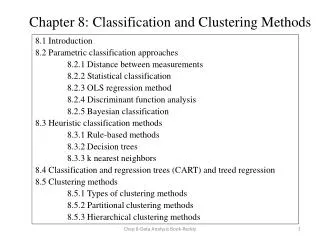
Chapter 8: Classification and Clustering Methods 8.1 Introduction 8.2 Parametric classification approaches 8.2.1 Distance between measurements 8.2.2 Statistical classification 8.2.3 OLS regression method 8.2.4 Discriminant function analysis 8.2.5 Bayesian classification 8.3 Heuristic classification methods 8.3.1 Rule-based methods 8.3.2 Decision trees 8.3.3 k nearest neighbors 8.4 Classification and regression trees (CART) and treed regression 8.5 Clustering methods 8.5.1 Types of clustering methods 8.5.2 Partitional clustering methods 8.5.3 Hierarchical clustering methods Chap 8-Data Analysis Book-Reddy

8.1 Introduction Clustering analysis involves several procedures by which a group of samples (or multivariate observations) can be clustered or partitioned or separated into sub-sets of greater homogeneity, i.e., those based on some pre-determined similarity criteria. • Examples: - clustering individuals based on their similarities with respect to physical attributes or mental attitudes or medical problems; - multivariate performance data of a mechanical piece of equipment can be separated into those which represent normal operation as against faulty operation. Thus, clustering analysis reveals inter-relationships between samples which can serve to group them under situations where one does not know the number of sub-groups beforehand. Often clustering results depend to largely on the clustering method used Chap 8-Data Analysis Book-Reddy

Classification analysis, applies to situations when the groups are known beforehand. • The intent is to identify models which best characterize the boundaries between groups, so that future objects can be allocated into the appropriate group. • Since the groups are pre-determined, classification problems are somewhat simpler to analyze than clustering problems. • The challenge in classification modeling is dealing with the misclassification rateof objects • Three types of classification methods are briefly treated: - parametric methods (involving statistical, ordinary least squares, discriminant analysis and Bayesian techniques), -heuristic methods (rule-based, decision-tree, k nearest neighbors) - parametric models (classification and regression trees) Chap 8-Data Analysis Book-Reddy

8.2 Parametric classification approaches Chap 8-Data Analysis Book-Reddy

Example 8.2.1. Using distance measures for evaluating canine samplesA biologist wishes to evaluate whether the modern dog in Thailand descended from prehistoric ones from the same region or were inbred with similar dogs which migrated from nearby China or India. The basis of this evaluation will be six measurements all related to the mandible or lower jaw of the dog: x1 – breadth of mandible, x2 – height of mandible below the first molar, x3 – length of first molar, x4 – breadth of first molar, x5 – length from first to third molar, x6 – length from first to fourth premolar. Chap 8-Data Analysis Book-Reddy

The measurements have to be standardized, and so, the mean and standard deviations for each variable across groups is determined . For example, the standardized value for the modern dog: z1= (9.7-11.25)/1.68=-0.922, and so on. Chap 8-Data Analysis Book-Reddy

Finally the Euclidean distances among all groups are computed as shown. It is clear that prehistoric dogs are similar to modern ones because their distances are much smaller than those of others. Next in terms of similarity are the Chinese and Indian wolfs. • Other measures of distance: • Manhattan measure: based on absolute measure • Mahanabolis measure: superior when variables are correlated Chap 8-Data Analysis Book-Reddy

8.2.2 Statistical classification ,Classification methods provide the necessary methodology to: • statistically distinguish or “discriminate” between differences in two or more groups when one knows beforehand that such groupings exist, and • subsequently assign a future unclassified observation into a specific group with the smallest probability of error. Fig. 8.1 Errors of misclassification for the univariate case. • When the two distributions are similar and if equal misclassification rates are sought, then the cutoff value or score is selected at the intersection point of the two distributions; • When the two distributions are not similar, a similar cut-off value will result in different misclassification errors. Chap 8-Data Analysis Book-Reddy

Example 8.2.2. Statistical classification of office buildings The objective is to distinguish between medium-sized office buildings which are ordinary (type O) or energy efficient (type E) To be judged by their “energy use index” (or EUI) First 10 values (C1 to C10) used to train (to determine the cut-off score), while the last four will be used for testing (to determine the misclassification rate) Chap 8-Data Analysis Book-Reddy

A simple first attempt at determining this value is to take it as being the mid-point of both the means. -Average values: for the first five buildings (C1-C5 are type O): 39.0 second five (C6-C10 are type E): 36.8 • If an average cut-off value of 38.2 is selected, one should expect the EUI for ordinary buildings to be higher than this value and that for energy efficient ones to be lower. • The results listed in the last column of Table 8.4 indicate one misclassification in each category during the training phase. • Thus, this simple-minded cutoff value may be acceptable since it leads to equal misclassification rates among both categories. • Note that among the last 4 buildings (C11-C14) used for testing the selected cut-off score, one of the ordinary buildings is improperly classified. Chap 8-Data Analysis Book-Reddy

Classification using the simple distance measure: Two groups are shown in Fig. 8.2 with normalized variables. • During training, centers and separating boundaries of each class are determined. - The two circles (shown continuous) encircle all the points. • A future observation will be classified in the group whose class center is closest However, a deficiency is that some of the points will be misclassified. • One solution to decreasing the misclassification rates is to reduce the boundaries (shown by dotted circles). • However, some of the observations now fall outside the dotted circles, and these points cannot be classified into either Class A or Class B. • Hence, the option of reducing the boundary diameters is acceptable if one is willing to group certain points into a third class called “unable to classify”. Fig. 8.2 Bivariate classification using the distance approach showing the centers and boundaries of the two groups. Chap 8-Data Analysis Book-Reddy

8.2.3 Ordinary Least Squares regression method Regression methods can also be used to model differences between groups and thereby assign a future observation to a particular group. - During regression, response variable is a continuous one -During classification, “ must be (or be converted) to categorical (regressors may be continuous or discrete or mixed) Fig. 8.3 Classification involves identifying a separating boundary between two known groups (shown as dots and crosses) based on two attributes (or variables or regressors) x1 and x2 which will minimize the misclassification of the points. Chap 8-Data Analysis Book-Reddy

Linear decision boundaries • Piecewise linear decision boundaries Fig. 8.4 Linear and piecewise linear decision boundaries for two-dimensional data (color intensity and alcohol content) used to classify the type of wine into one of three classes Chap 8-Data Analysis Book-Reddy

8.2.4 Discriminant Function Analysis Method optimal when the two classes are normally distributed with equal covariance matrices; even when they are not, the method gives satisfactory results. Chap 8-Data Analysis Book-Reddy

Chap 8-Data Analysis Book-Reddy

Table 8.5 Analysis results for chiller fault detection example using two different methods: OLS regression and the linear discriminant analysis (LDA) Portion of table Chap 8-Data Analysis Book-Reddy

Example 8.2.3. Using discriminant analysis to distinguish fault-free and faulty behavior of chillers MLR and LDA used to classify two data sets representative of normal and faulty operation of a large centrifugal chiller using three regressors variables. The two data sets consist of 27 operating points each; however, 21 points are used for training the model while the remaining points are used for evaluating the classification model. Fault-free data is assigned a class value of 0 while faulty data a value of 1. Models identified from training data used to predict class membership for testing data. The cut-off score is 0.5 for both approaches, i.e., if calculated score is less than 0.5, then the observation is deemed to belong to the fault-free behavior, and vice versa. Chap 8-Data Analysis Book-Reddy

Fig. 8.5 Scatter plot of the three variables. Fault-free data (coded 0) is shown as diamonds while faulty data (coded 1) is shown as crosses. Clearly there is no overlap between the data sets and the analysis indicates no misclassified data points. Chap 8-Data Analysis Book-Reddy

Fig 8.6 Though an OLS model can be used for classification, it is not really meant for this purpose. This is illustrated by the poor correspondence between observed vs predicted values of the coded “class” variables. The observed values can assume numerical values of either 0 or 1 only, while the values predicted by the model range from -0.2 to about 1.2 Chap 8-Data Analysis Book-Reddy

Summary of example results: LDA model scores also fall on either side of 0.5 but are magnified as compared to the OLS scores leading to more robust classification. In this example, there are no misclassification data points for either model during both training and testing periods. Several studies use standardized regressors (with zero mean and unit variance) to identify the discriminant function. Others argue otherwise. One difference is that when using standardized variables, the discriminant function would not need an intercept term, while this is needed when using untransformed variables. Though LDA is widely used for classification problems, it is increasingly being replaced by logistic regression since the latter: - makes fewer assumptions on distribution of variables (so more flexible) - more robust statistically when dealing with actual data. - more parsimonious - value of the weights easier to interpret. A drawback (if it is one!) is that model weights have to be estimated by maximum likelihood method Chap 8-Data Analysis Book-Reddy

8.2.5 Bayesian Classification Recall: Bayesian statistics provide the formal manner by which prior opinion expressed as probabilities can be revised in the light of new information (from additional data collected) to yield posterior probabilities. It can also be used for classification tasks . The simplified or Naïve Bayesmethod assumes that the predictors are statistically independent and uses prior probabilities for training the model, which subsequently can be used along with the likelihood function of a new sample to classify the sample into the most likely group. • Advantages: training and classification are easily interpreted, can handle large number of predictors, easy to use, handles missing data well, requires little computational effort. • Disadvantages: does not handle continuous data well does not always yield satisfactory results. Despite these limitations, it is a useful analysis approach to have in one’s toolkit. Chap 8-Data Analysis Book-Reddy

Example 8.2.4. Bayesian classification of coal sample based on carbon content A power plant gets two types of coal: bituminous and anthracite. Each of these two types can contain different fixed carbon content depending on the time at which and the location from where the sample was mined. Further, each of these types of coal can be assigned into one of three categories: Poor, Average and Good depending on the carbon content whose thresholds are different for the two types of coal. For example, a bituminous sample can be graded as “good” while an anthracite sample can be graded as “average” even though both samples may have the same carbon content. Training Data Set Chap 8-Data Analysis Book-Reddy

The power plant operator wants to classify a new sample of bituminous carbon which is found to contain 70-80% carbon content. • The sample probabilities are shown in the third column of the table below. • The values in the likelihood column add up to 0.0332 which is used to determine the actual posterior probabilities shown in the last column. • The category which has the highest posterior probability can then be identified. • Thus, the new sample will be classified as “average”. Chap 8-Data Analysis Book-Reddy

8.3 Heuristic Classification Methods • 8.3.1 Rule Based Methods • Simplest method: uses “if-then” rules. • Such classification rules consist of the “if” or antecedent part and the “then” or consequent part of the rule. • These rules must cover all the possibilities, and every instance must be uniquely assigned to a particular group. • Such a heuristic approach is widely used in several fields because of the ease of interpretation and implementation of the algorithm. Chap 8-Data Analysis Book-Reddy

For example, consider an applicant with UA GPA=3.6 and MCAT-V =525. He would fall under group D and be rejected without an interview. Thus, the pre-determined threshold or selection criteria of GPA, MCAT-V and MCAT-Q are in essence the classification model, while classification of a future applicant is straightforward. Chap 8-Data Analysis Book-Reddy

8.3.2 Decision Trees Similar to probability trees Graphical way of dividing a decision problem into a hierarchical structure for easier understanding and analysis. Decision trees are predictive modeling approaches which can be used for classification, clustering as well as for regression model building. They essentially divide the spatial space such that each branch can be associated with a different sub-region. A rule is associated with each node of the tree, and observations which satisfy the rule are assigned to the corresponding branch of the tree. Though similar to if-then rules in their structure, decision trees are easier to comprehend in more complex situations, and are more efficient computationally. Fig. 8.7 Tree diagram for the medical school admission process with five terminal nodes, each representing a different group. This is a binary tree with three levels. How an applicant pool of 727 are screened at each stage is shown Chap 8-Data Analysis Book-Reddy

8.3.3 k Nearest Neighbors (kNN) • (kNN) is a conceptually simple approach widely used for classification. • It is based on the distance measure, and requires a training data set of observations from different groups identified as such. • A future object can be classified by determining the point closest to this new object, and simply assigning the new object to the group to which the closest point belongs. The classification is more robust if a few points are used rather than a single closest neighbor. This, however, leads to the following issues which complicate the classification: • how many closest points “k” should be used for the classification, and • how to reconcile differences when nearest neighbors come from different groups. kNN is more of an algorithm than a clear-cut analytical procedure. An allied classification method is the closest neighborhoodscheme, where an object is classified in that group for which its distance from the center of that group happens to be the smallest as compared to its distances from the centers of other possible groups. Training would involve computing the centers of each group and distances of individual objects from this center. • A redeeming feature of kNN is that it does not impose a priori any assumptions about the distribution from which the modeling sample is drawn. Chap 8-Data Analysis Book-Reddy

Fig. 8.8 Illustration of the neighborhood concept for a baseline with two regressors (dry-bulb temperature DBT and dew point temperature DPT) If the DBT variable has more “weight” than DPT on the variation of the response variable, this would translate geometrically into an elliptic domain as shown. The data set of “neighbor points” to the post datum point (75, 60) would consist of all points contained within the ellipse. Further, a given point within this ellipse may be assigned more “influence” the closer it is to the center of the ellipse (from Subbarao et al., 2011). Chap 8-Data Analysis Book-Reddy

The approach is illustrated with a simple example involving synthetic daily data of building energy use. Only two variables are considered: regressors: ambient air dry-bulb temperature (DBT) and dew point temperature (DPT) Fig. 8.9 Scatter plot of thermal cooling load Qc versus DBT Chap 8-Data Analysis Book-Reddy

8.4 Classification and Regression Trees (CART) • Constructing a tree is analogous to training in a model-building context, but here, it involves : (i) choosing the splitting attributes, i.e., the set of important variables to perform the splitting; in many engineering problems, this is a moot step, (ii) ordering the splitting attributes, i.e., ranking them by order of importance in explaining the variation in the dependent variable, (iii) deciding on the number of splits of the splitting attributes which is dictated by the domain or range of variation of that particular attribute, (iv)defining the tree structure, i.e., number of nodes and branches, (v) selecting stopping criteria which are a set of pre-defined rules which reveal that no further gain is being made in the model; (vi) pruning which involves making modifications to the tree constructed using the training data so that it applies well to the testing data. Chap 8-Data Analysis Book-Reddy

(CART) is a non-parametric decision tree technique that can be applied either to classification or regression problems, depending on whether the dependent variable is categorical or numeric respectively • It is one of an increasing number of computer intensive methods which perform an exhaustive search to determine best tree size and configuration in multivariate data. While being a fully automatic method, it is flexible, powerful and parsimonious, i.e., it identifies a tree with the fewest number of branches. • Another appeal of CART is that it chooses the splitting variables and splitting points that best discriminate between the outcome classes. The algorithm, however, suffers from the danger of over-fitting, and hence, a cross-validation data set is essential Chap 8-Data Analysis Book-Reddy

Most trees, including CART are binary decision trees (i.e., the tree splits into two branches at each node), though this is not mandatory • Each branch of the tree ends in a terminal node while each observation falls into one and exactly one terminal node. • The tree is created by an exhaustive search performed at each node to determine the best split. The computation stops when any further split does not improve the classification. • Treed regression is very similar to CART except that the latter fits the mean of the dependent variable in each terminal node, while treed regression can assume any functional form. Chap 8-Data Analysis Book-Reddy

Example 8.4.1. Using treed regression to model atmospheric ozone variation with climatic variables. Cleveland (1994) presents data from 111 days in the New York City metropolitan region in the early 1970s consisting of: - ozone concentration (an index for air pollutant) in parts per billion (ppb), and three climatic variables: ambient temperature (in 0F), wind speed (in mph) and solar radiation (in langleys). It is the intent to develop a regression model for predicting ozone levels against the three variables. One notes that though some sort of correlation exits, the scatter is fairly important. An obvious way is to use multiple regression with inclusion of higher order terms as necessary. Fig. 8.10(a) Scatter plots of ozone versus climatic data Chap 8-Data Analysis Book-Reddy

Fig. 8.10(b) Scatter plots and linear regression models for the three terminal nodes of the treed regression model Chap 8-Data Analysis Book-Reddy

Fig. 8.10(c) Treed regression model for predicting ozone level against climatic variables Chap 8-Data Analysis Book-Reddy

CART and treed regression are robust methods which are ideally suited for the analysis of complex data which can be numeric or categorical, involving nonlinear relationships, high-order interactions, and missing values in either response or regressor variables. • Despite such difficulties, the methods are simple to understand and give easily interpretable results. • Trees explain variation of a single response variable by repeatedly splitting the data into more homogeneous groups or spatial ranges, using combinations of explanatory variables that may be categorical and/or numeric. • Each group is characterized by a typical value of the response variable, the number of observations in the group, and the values of the explanatory variables that define it. • The tree is represented graphically, and this aids exploration and understanding. Classification and regression have a wide range of applications, including scientific experiments, medical diagnosis, fraud detection, credit approval, and target marketing Chap 8-Data Analysis Book-Reddy

8.5 Clustering Methods Aim of cluster analysis is to allocate a set of observation sets into groups which are similar or “close” to one another with respect to certain attribute(s) or characteristic(s). Thus, an observation can be placed in one and only one cluster. For example, performance data collected from mechanical equipment could be classified as representing good, faulty or uncertain operation. • In general, the number of clusters is not predefined and has to be gleaned from the data set. • This and the fact that one does have a training data set to build a model make clustering a much more difficult problem than classification. • A wide variety of clustering techniques and algorithms has been proposed, and there is no generally accepted best method. • Some authors point out that, except when the clusters are clear-cut, the resulting clusters often depend on the analysis approach used and somewhat subjective. • Thus, there is often no one single best result, and there exists the distinct possibility that different analysts will arrive at different results. Chap 8-Data Analysis Book-Reddy

Broadly speaking, there are two types of clustering methods both of which are based on distance-algorithms where objects are clustered into groups depending on their relative closeness to each other. • partitional clustering where non-overlapping clusters are identified. • hierarchic clustering which allows one to identify closeness of different objects at different levels of aggregation. Thus, one starts by identifying several lower-level clusters or groups, and then gradually merging these in a sequential manner depending on their relative closeness, so that finally only one group results. Both approaches rely, in essence, in identifying those which exhibit small within-cluster variation as against large between-cluster variation. Several algorithms are available for cluster analysis Chap 8-Data Analysis Book-Reddy

Partitional clustering (or disjoint clusters) determines the optimal number of clusters by performing the analysis with different pre-selected number of clusters A widely used criterion is the within-cluster variation, i.e., squared error metric which measures the square distance from each point within the cluster to the centroid of the cluster. Similarly, a between-cluster variation can be computed representative of the distance from one cluster center to another. The ratio of the between-cluster variation to the average within clusters is analogous to the F-ratio used in ANOVA tests. Thus, one starts with an arbitrary number of cluster centers, start assigning objects to what is deemed to be the nearest cluster center, compute the F-ratio of the resulting cluster, and then jiggle the objects back and forth between the clusters each time re-calculating the mean so that the F ratio is maximized or is sufficiently large. It is recommended that this process be repeated with different seeds or initial centers since their initial selection may result in cluster formations which are localized. This tedious process can only be done by computers for most practical problem. A slight deviant of the above algorithm is the widely used k-means algorithm where instead of a F-test, the sum of the squared errors is directly used for clustering. This is best illustrated with a simple two-dimension sample. Chap 8-Data Analysis Book-Reddy

8.5.2 Partitional Clustering methods Determines the optimal number of clusters by performing the analysis with different pre-selected number of clusters A widely used criterion is the within-cluster variation, i.e., squared error metric which measures the square distance from each point within the cluster to the centroid of the cluster. Similarly, a between-cluster variation can be computed representative of the distance from one cluster center to another. The ratio of the between-cluster variation to the average within clusters is analogous to the F-ratio used in ANOVA tests. Fig. 8.11 Schematic of two clusters with individual points shown as x. The within-cluster variation is the sum of the individual distances from the centroid to the points within the cluster, while the between-cluster variation is the distance between the two centroids Chap 8-Data Analysis Book-Reddy

Algorithm • Start with an arbitrary number of cluster centers, • Assign objects to what is deemed to be the nearest cluster center, • Compute the F-ratio of the resulting cluster, • Jiggle the objects back and forth between the clusters each time re-calculating the mean so that the F ratio is maximized or is sufficiently large. It is recommended that this process be repeated with different seeds or initial centers since their initial selection may result in cluster formations which are localized. This tedious process can only be done by computers for most practical problem. A slight deviant of the above algorithm is the widely used k-means algorithmwhere instead of a F-test, the sum of the squared errors is directly used for clustering. This is best illustrated with a simple two-dimension sample. Chap 8-Data Analysis Book-Reddy

9.36 Chap 8-Data Analysis Book-Reddy

Fig. 8.12 Visual clustering may not always lead to an optimal splitting Chap 8-Data Analysis Book-Reddy

8.5.3 Hierarchical Clustering Methods Hierarchical clustering, does not start by partitioning a set of objects into mutually exclusive clusters, but forms them sequentially in a nested fashion. For example, the eight objects shown at the left of the tree diagram (also called dendrogram) are merged into clusters at different stages depending on their relative similarity. This allows one to identify objects which are close to each other at different levels. Chap 8-Data Analysis Book-Reddy

Chapter 8: Classification and Clustering Methods