Download
1 / 23
230 likes | 494 Views
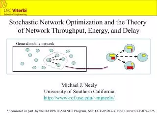
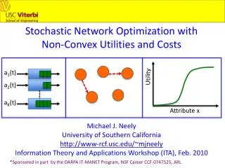
Stochastic Network Optimization with Non-Convex Utilities and Costs. a 1 (t). Utility. a 2 (t). a K (t ). Attribute x. Michael J. Neely University of Southern California http://www-rcf.usc.edu/~mjneely Information Theory and Applications Workshop (ITA), Feb. 2010.

E N D
Stochastic Network Optimization with Non-Convex Utilities and Costs a1(t) Utility a2(t) aK(t) Attribute x Michael J. Neely University of Southern California http://www-rcf.usc.edu/~mjneely Information Theory and Applications Workshop (ITA), Feb. 2010 *Sponsored in part by the DARPA IT-MANET Program, NSF Career CCF-0747525, ARL
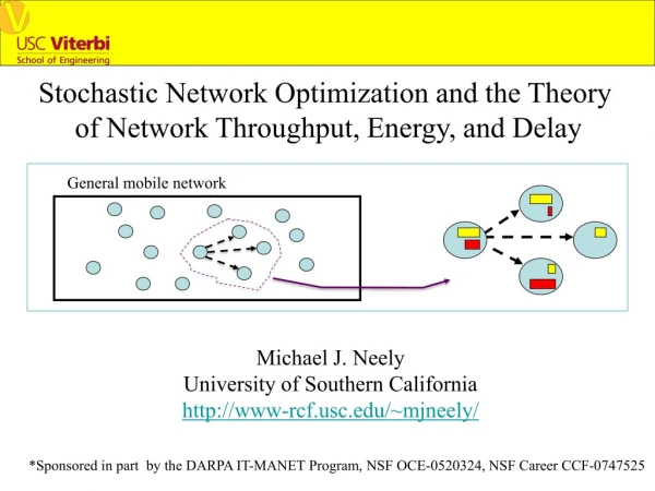
ak(t) bk(t) • Problem Description: • K Queue Network --- (Q1(t), …, QK(t)) • Slotted time, t in {0, 1, 2, … } • w(t) = “Random Network Event” (e.g., arrivals, channels, etc.) • a(t) = “Control Action” (e.g., power allocation, routing, etc.) • Decision: • Observe w(t) every slot. Choose a(t) in Aw(t). • Affects, arrivals, service, and “Network Attributes”: • ak(t) = ak(w(t),a(t)) = arrivals to queue k on slot t • bk(t) = bk(w(t),a(t)) = service to queue k on slot t • xm(t) = xm(w(t),a(t)) = Network Attribute mon slot t (these are general functions, possibly non-convex, discontinuous)
What are “Network Attributes” ? • x(t) = (x1(t), …, xM(t)) • Traditional: • Packet Admissions / Throughput • Power Expenditures • Packet Drops • Emerging Attributes for Network Science: • Quality of Information (QoI) Metrics • Distortions • Profit • Real-Valued Meta-Data
Define Time Averages: • x = ( x1 , …, xM) • Goal: • Minimize : f( x ) • Subject to: 1) gn( x ) ≤ 0 for n in {1, …, N} • 2) x in X • 3) All queues Qk(t) stable • Where: • X is an abstract convex set • gn(x) are convex functions • f(x) is a possibly non-convex function!
Example Problem 1: Maximizing non-concave thruput-utility x = ( x1 , …, xM) = time avg “thruput” attribute vector f(x) = Non-Concave Utility = f1(x1) + f2(x2) + … + fM(xM) Utility fm(x) Attribute x Utility is only large when thruput exceeds a threshold. Global Optimality can be as hard as combinatorial bin-packing.
Example Problem 2: Risk-Aware Networking (Variance Minimization) Let p(t) = “Network Profit” on slot t. Define Attributes: x1(t) = p(t) x2(t) = p(t)2 Then: Var(p) = E{p2} – E{p}2 = x2 – ( x1 )2 Minimizing variance minimizes a non-convex function of a time-average! Non-Convex!
Prior Work on Non-Stochastic (static) Non-Convex • Network Optimization: • Lee, Mazumdar, Shroff, TON 2005 • Chiang 2008 Utility fm(x) Attribute x
Prior Work on Stochastic, Convex Network Optimization: • Dual-Based: • Neely 2003, 2005, Georgiadis, Neely, Tassiulas F&T 2006 • Explicit optimality, performance, convergence analysis via a • “drift-plus-penalty” alg: [O(1/V), O(V)] Performance-Delay tradeoff • Eryilmaz, Srikant 2005 (“fluid model,” infinite backlog) • Primal-Dual-Based: • Agrawal, Subramanian 2002 (no queues, infinite backlog) • Kushner, Whiting 2002 (no queues, infinite backlog) • Stolyar 2005, 2006 (with queues, but “fluid model”): • Proves optimality over a “fluid network.” • Conjectures that the actual network utility approaches • optimal when a parameter is scaled.
Summary: • 1) Optimizing a time average of a non-convex function is Easy! • (can find global optimum Georgiadis, Neely, Tassiulas F&T 2006). • 2) Optimizing a non-convex function of a time average is Hard! • (CAN WE FIND A LOCAL OPTIMUM??) • Drift-Plus-Penalty with “Pure-Dual” Algorithm: • Works great for convex problems • Robust to changes, has explicit performance, convergence bounds • BUT: For non-convex problems, it would find global optimum of • the time average of f(x), which is not necessarily • even a local optimum of f( x ). • Drift-Plus-Penalty with “Primal-Dual” Component: • OUR NEW RESULT: Works well for non-convex! • Can find a local optimum of f( x )!
Solving the Problem via a Transformation: Original Problem: Min: f( x ) Subject to: 1) gn( x ) ≤ 0 , n in {1,…,N} 2) x in X 3) All Queues Stable Transformed Problem: Min: f( x ) Subject to: 1) gn( g ) ≤ 0 , n in {1,…,N} 2) gm = xm , for all m 3) g(t) in X , for all t 4) All Queues Stable Auxiliary Variables: g(t) =(g1(t), …, gM(t)). These act as a proxy for x(t) = (x1(t), …, xM(t)). Constraints in the new problem are time averages of functions, not functions of time averages! And the problems are equivalent!
Solving the Problem via a Transformation: Next Step: Lyapunov Optimization: Transformed Problem: Min: f( x ) Subject to: 1) gn( g ) ≤ 0 , n in {1,…,N} 2) gm = xm , for all m 3) g(t) in X , for all t 4) All Queues Stable • Define Virtual Queue for each inequality and equality constraint • Q(t) = vector of virtual and actual queues. • Use Quadratic Lyapunov function, Drift = D(t) • Use Min Drift-Plus-Penalty… Auxiliary Variables: g(t) =(g1(t), …, gM(t)). These act as a proxy for x(t) = (x1(t), …, xM(t)). Constraints in the new problem are time averages of functions, not functions of time averages! And the problems are equivalent!
Use a “Primal” Derivative in Drift-Plus-Penalty: • Every slot t, observe w(t) and current queues Q(t). • Choose a(t) in Aw(t), a(t) in X to minimize… ∂ f( x(t) ) xm(w(t),a(t)) D(t) + V ∂ xm m where x(t) = (x1(t), …., xM(t)) = Empirical Running Time Avg. up to time t (starting from time 0) • Doesn’t need knowledge of traffic or channel statistics! • Can “approx” minimize to within constant C of infimum. Note: “Pure Dual” Algorithm Minimizes D(t) + Vf(g(t)), does not need running time average, is more robust to varying parameters and provides stronger guarantees, but only works for convex f() functions!
∂ f( x(t) ) xm(w(t),a(t)) D(t) + V ∂ xm m Theorem: Assuming the constraints are feasible, then for any parameter choice V ≥ 0, we have: All required constraints are satisfied. All queues strongly stable with: E{Delay} ≤ O(V) Assuming the attribute vector converges with prob. 1, then Time Average Attribute vector is a “Near-Local-Min”: ∂ f( x ) (xm - xm) ≥ -(B +C)/V * ∂ xm m where x* = (x1*, …, xM*) is any other feasible time average vector
Proof Sketch: Very Simple Proof! Because we take actions to minimize the drift-plus-penalty every slot (given current queue states) to within C, we have: ∂ f( x(t) ) xm(w(t),a(t)) D(t) + V ∂ xm m ∂ f( x(t) ) xm(w(t), a*(t)) D*(t) + V ≤ C + ∂ xm m where D*(t) and a*(t) are the drift and decision under any other (possibly randomized) decision choices! But for any feasible time average vector x*, there are choices that make the drift zero (plus a constant B that is Independent of queue state)…so….
Proof Sketch: Very Simple Proof! Because we take actions to minimize the drift-plus-penalty every slot (given current queue states) to within C, we have: ∂ f( x(t) ) xm(w(t),a(t)) D(t) + V ∂ xm m xm * B ∂ f( x(t) ) xm(w(t), a*(t)) D*(t) + V ≤ C + ∂ xm m where D*(t) and a*(t) are the drift and decision under any other (possibly randomized) decision choices! But for any feasible time average vector x*, there are choices that make the drift zero (plus a constant B that is Independent of queue state)…so….
Proof Sketch: Very Simple Proof! Because we take actions to minimize the drift-plus-penalty every slot (given current queue states) to within C, we have: ∂ f( x(t) ) xm(w(t),a(t)) D(t) + V ∂ xm m ∂ f( x(t) ) * xm ≤ C + B + V ∂ xm m • The rest follows by (see [Georgiadis, Neely, Tassiulas, F&T 2006)]: • Iterated Expectations: E{E{X|Y}} = E{X} • Telescoping Sums: • [f(4) – f(3)] + [f(3) –f(2)] + [f(2) – f(1)] + [f(1) – f(0)] = f(4) – f(0) • Rearranging Terms and Taking Limits
Extension 1: Using a “Variable V(t)” algorithm with increasing V(t): V(t) = (1+t)d (for 0 < d < 1) gives a true local min: ∂ f( x ) (xm - xm) ≥ 0 * ∂ xm m where x* = (x1*, …, xM*) is any other feasible time average vector All Constraints are still satisfied with this Variable-V algorithm. However, queues are only “mean rate stable” (input rate = output rate) and have infinite average congestion and delay!
Extension 2: A 3-phase algorithm in special case when Utility function f(x) is entrywise non-decreasing: Phase 1: Pick Directions {q1, …, qN}. Solve the convex stochastic net opt problem via pure dual method: Maximize: b Subject to: 1) x = bqn 2) desired constraints 3) All queues stable Unknown “Attribute Region” Phase 2: Solve (to a local min) the deterministic problem: Max: f(x1,…,xM) S.t.: (x1,…, xM) in Conv{b1q1, …,bnqn} optimal x*
Extension 2: A 3-phase algorithm in special case when Utility function f(x) is entrywise non-decreasing: Phase 3: Solve the convex stochastic net opt problem via pure dual method: Maximize: b Subject to: 1) x = bx* 2) desired constraints 3) All queues stable x* This involves 1 purely deterministic non-convex phase (any static solver can be used) and 2 purely convex stochastic network optimizations!
Conclusions: • We have studied techniques for non-convex stochastic • network optimization. • “Primal-Dual” partial derivative info used with • Drift-Plus-Penalty metric for achieving local min. • Requires a running time average, not as robust to • changes, convergence time issues unclear • Second approach uses 3-phases, the stochastic parts • are purely convex, and we can use the pure-dual method • to provide stronger performance guarantees.
Some Possible Questions: • 1) Why do we use auxiliary variables? • They allow treatment of the abstract set • constraint • They allow the constraints of the problem • to be transformed into constraints on time • averages of functions, rather than functions • of time averages. • This enables explicit bounds on convergence • times. • It also ensures the constraint satisfaction • is robust to system changes, even if the • non-convex utility optimization is not.
Some Possible Questions: • 2) How is the first method different from • prior stochastic primal-dual methods? • We use auxiliary variables • We treat the convex inequality constraints via • a “pure-dual” (no derivatives) to get stronger • proof that all constraints are met, and to within • a known convergence time • We treat abstract set constraints • We treat the non-convex problem (the lack of • convergence time knowledge for the utility part • is due to the “primal” component, but this is • the price of treating non-convex problems!) • We treat joint queue stability and utility optimization, • with a proof that is even simpler than the fluid limit • proof given for the special case of convex problems in • Stolyar 05, 06.
Some Possible Questions: • 3) Why do we consider the 3-phase algorithm? • Uses 2 pure convex stochastic problems (and • so the stochastic parts have stronger and • more explicit convergence time guarantees, do • not require derivatives to exist). • The 1 non-convex optimization is a pure • deterministic problem, from which we can use • any known deterministic solver (such as “brute • force,” or “Nelder-Mead,” or “Newton-type” • methods that do not necessarily restrict to small • step sizes.