Download

1 / 25
270 likes | 615 Views
Nonlinear Oscillations; Chaos Mainly from Marion, Chapter 4. Confine general discussion to oscillations & oscillators. Most oscillators seen in undergrad mechanics are Linear Oscillators: Obey Hooke’s “Law”, linear restoring force: F(x)= -kx Potential energy V(x)= (½)kx 2

E N D
Nonlinear Oscillations; ChaosMainly from Marion, Chapter 4 • Confine general discussion to oscillations & oscillators. Most oscillators seen in undergrad mechanics are Linear Oscillators: Obey Hooke’s “Law”, linear restoring force: F(x)= -kx Potential energy V(x)= (½)kx2 • Real world: Most oscillators are, in fact,nonlinear! • Techniques for solving linear problems might or might not be useful for nonlinear ones! • Often, rather than having a general technique for nonlinear problem solution, technique may be problem dependent. • Often need numerical techniques to solve diff. eqtns.
Many techniques exist for solving (or at least approximately solving) nonlinear differential equations. • Often, nonlinear systems reveal a rich & beautiful physics that is simply not there in linear systems. (e.g. Chaos). • The related areas of nonlinear mechanics and Chaos are very modern & are (in some places) hot topics of current research! • I am not an expert!
Nonlinear Oscillations • Consider a general 1 d driven, damped oscillator for which Newton’s 2nd Law equation of motion is:(v = dx/dt) m(d2x/dt2) + f(v)+ g(x) = h(t) (1) • f(v), g(x),h(t) problem dependent! • If f(v) contains powers of v higher than linear & / or g(x) contains powers of x higher than linear, (1) is a non-linear differential equation. • Complete, general solutions are not always available! • Sometimes special treatment adapted for a problem is needed. • Can learn a lot by considering deviations from linearity. • Sometimes examining the phase (v-x) diagrams is useful.
A Brief History & Terminology:The Early 1800’s:Laplace’s idea:N’s 2nd Law. If at t = 0 positions & velocities of all particles in universe are known, & if force laws governing particle interactions are known, then we can know theexact future of the universe by integrating N’s 2nd Law equations. A Deterministicview of nature.Recently:In the past 35 years or so, researchers in many (different) areas of science have realized that knowing the laws of nature is not enough. Much of nature ischaotic! Deterministic Chaos:Motion of a system whose time evolution dependssensitively initial conditions. Deterministic:For given initial conditions, N’s 2nd Law equations give the exact future of the system.Chaos:Only slight changes in initial conditions can result indrastic changesin the system motion.Random:There is no correlation between the system’s present state & it’s immediate past state.Chaos & randomness are different!
Chaos:Measurements on the system at given time might not allow the future to be predicted with certainty, even if the force laws are known exactly! (Experimental uncertainties in the initial conditions).Deterministic Chaos:Alwaysassociated with a systemnonlinearity.Nonlinearity:Necessary for chaos, but not sufficient!All chaotic systems are nonlinear but not all nonlinear systems are chaotic. • Chaos occurs when the system depends very sensitively on its previous state. Even a tiny change in initial conditions can completely change the system motion. • Chaotic Systems:Can only be solved numerically. Only with the availability of modern computers has it become possible to study these phenomena. No simple, general rules for when the system will be chaotic or not. Chaotic phenomena in the real world: Irregular heartbeats, Planet motion in the solar system, Electrical circuits, Weather patterns, …
Chaotic Systems: • Henri Poincaré: In the late 1800’s. The first to recognize chaos (in celestial mechanics). • Real breakthroughs in understanding came in the 1970’s (with computers). • Chaos study is widespread. We will only give a brief, elementary introduction. • Many textbooks and popular texts exist! See References to Goldstein’s Ch. 11 or Marion’s Ch. 4. • This is a very popular & popularized topic even in the mainstream, popular press.
Chaos in a Pendulum • Use the damped, driven pendulum to introduce Chaos concepts. • Pendulum:The nonlinearity has been known for hundreds of years. Chaotic behavior only known (& explored) recently. Some pendulum motions which are known to be chaotic: • Forced oscillating support:
Double pendulum: • Coupled pendula:
We aren’t going to analyze these! • Consider the ordinary pendulum, but add a driving torque (Nd cos(ωdt)) & a damping term (-b(dθ/dt)) • The Equation of Motion is obtained by equating the total torque around the pivot point with the moment of inertia the angular acceleration. N = I(d2θ/dt2) = - b(dθ/dt) -mgsinθ + Nd cos(ωdt)
Equation of motion: N = I(d2θ/dt2) = - b(dθ/dt) - mgsinθ + Nd cos(ωdt) Divide by I = m2 (d2θ/dt2) = - b(m2)-1(dθ/dt) - g()-1sinθ + Nd(m2)-1cos(ωdt) • Go to dimensionless variables (for ease of numerical solution): Divide eqtn by natural frequency squared: (ω0)2(g/) • Define dimensionless variables: Time: t ω0t (g/)½t Driving frequency:ω(ωd/ω0) (/g)½ωd Variable:x θ Damping constant: c b(m2ω0)-1 b(mg)-1 Driving force strength:F Nd(m2ω0)-1 Nd(mg)-1
To solve this numerically, its first convert this 2nd order differential equation to two 1st order diff. eqtns! x + cx + sin(x) = F cos(ωt).DEFINE: y (dx/dt) = x (angular velocity),z ωt (dy/dt) = - cy – sin(x) + F cos(z) • Results are shown in the rather complicated figure (next page), which we’ll now look at in detail! For c = 0.05, ω = 0.7, results are shown for (driving torque strength) F = 0.4, 0.5, 0.6, 0.7, 0.8, 0.9 • Bottom line of the results from the figure: 1. The motion is periodic for F = 0.4, 0.5, 0.8, 0.9 2. The motion is chaotic for F = 0.6, 0.7, 1.0 • This indicates the richness of the results which can come from nonlinear dynamics! This is surprising only if you think linearly! Thinking linearly, one would expect the solution for F = 0.6 to not be much different from that for F = 0.5, etc.
F = 0.8 • Left figure shows y (dx/dt)(angular velocity)vs time tat steady state (transient effects have died out). F = 0.4 ~ simple harmonic motion F = 0.5 periodic, but not very “simple”! F = 0.9 F = 0.6 F = 1.0 F = 0.7 F = 0.8, 0.9 are ~ similar toF = 0.5. F = 0.6, 0.7, 1.0 are VERY different from the others: CHAOS!
F = 0.8 Periodic again. One complete revolution + oscillation. • Middle figure shows x – (dx/dt) phase space plots for the same cases (periodic, so only -π < x < π is needed). F = 0.4 ~ ellipse, as expected for simple harmonic motion F = 0.5 Much more complicated! 2 complete revolutions & 2 oscillations! F = 0.6 & F = 0.7 Entire phase plane is accessed. A SIGN OF CHAOS! F = 0.9 2 different revolutions in one cycle (“period doubling”). F = 1.0: The entire phase plane is accessed again! A SIGN OF CHAOS!
F = 0.4 F = 0.8 • Right column: “Poincaré Sections”: Need lots of further explanation! F = 0.5 F = 0.9 F = 0.6 F = 1.0 F = 0.7
Poincaré Sections • Poincaré Sections:Poincaré invented a technique to simplify representations of complicated phase space diagrams, such as we’ve just seen. • They are essentially2d representations of 3d phase space diagram plots. In our case, the 3d are: y [= (dx/dt) = (dθ/dt)]vsx (= θ)vs z(= ωt). Left column of the first figure (angular velocity y vs. t) = the projection of this plot onto a y-z plane, showing points corresponding to various x. Middle column of the first figure = the projection onto a y-x plane, showing points belonging to variousz. • The figure on the next page shows a 3d phase space diagram, intersected by a set of y-x planes, perpendicular to the z axis & at equal z intervals.
Poincaré Sections Explanation follows!
Poincaré Section Plot: Or, simply, Poincaré SectionThe sequence of points formed by the intersection of the phase path • with these parallel planes in • phase space, projected onto • one of the planes. The phase • path pierces the planes as a • function of angular speed [y = (dθ/dt)], time (z ωt) & phase angle (x = θ). The points of intersection are labeled A1, A2, A3, etc. The resulting set of points {Ai}forms a PATTERN when projected onto one of the planes. Sometimes, the pattern is regular & recognizable, sometimes irregular. Irregularity of the pattern can be a sign of chaos.
Poincarérealized that 1. Simple curves generated like this represent regular motion with possibly analytic solutions, such as the regular curves for F = 0.4 & 0.5 in the driven pendulum problem. 2.Many complicated, irregular, curves represent CHAOS! • Poincaré Section: Effectively reduces an N dimensional diagram to N-1 dimensions for graphical analysis. Can help to visualize motion in phase space & determine if chaos is present or not.
F = 0.4 0.5 0.6 • F = 0.5Poincaré Section has 3 points, because of more complex motion. • In general, the number of points n in the Poincaré Sectionshows that the motion is periodic with a period different than the period of the driving force. In general this period is T = T0(n/m), where T0 = (2/ω) is period of the driving force & m = integer. (m = 3 for F = 0.5) 0.7
F = 0.8 0.9 • F = 0.8: The Poincaré Sectionagain has only 1 point (“simple”, regular motion.) • F = 0.9: 2 points (more complex motion). T = T0(n/m), m = 2. • F = 0.6, 0.7, 1.0:CHAOTIC MOTION & new period T . The Poincaré Section is rich in structure! 1.0
Recall from earlier discussion: • ATTRACTORA set of points (or one point) in phase space towards which a system motion converges when damping is present. When there is an attractor, the regions traversed in phase space are bounded. • For Chaotic Motion,trajectories which are very near each other in phase space are diverging from one another. However, they must eventually return to the attractor. • Attractors in chaotic motion Strange Attractors or Chaotic Attractors.
Because Strange Attractors are bounded in phase space, they must fold back into the nearby phase space regions. Strange Attractors create intricate patterns, as seen in the Poincaré Sectionsof the example we’ve discussed. Because of the uniqueness of the solutions to the Newton’s 2nd Law differential equations, the trajectories must still be such that no one trajectory crosses another. • It is also known, that some of these Strange or Chaotic Attractors areFRACTALS!