Download
1 / 94
940 likes | 1.13k Views
Gamma-ray Large Area Space Telescope. GLAST and pulsars: models and simulations. Massimiliano Razzano (INFN-Pisa). Astrofisica gamma dallo spazio in Italia AGILE e GLAST ESRIN, Frascati, 3 luglio 2007. PulsarSpectrum, simulating pulsars for GLAST. Main Features

E N D
Gamma-ray Large Area Space Telescope GLAST and pulsars:models and simulations Massimiliano Razzano (INFN-Pisa) Astrofisica gamma dallo spazio in Italia AGILE e GLAST ESRIN, Frascati, 3 luglio 2007 M.Razzano
PulsarSpectrum, simulating pulsars for GLAST Main Features Provide realistic simulations to help developing and testin analysis tools and techniques Flexible architecture to allow creation of pulsar sources; Pulsar parameters easy to implement; PSRPhenom: Phenomenological model; PSRShape: Simulation of arbitrary energy-phase photon distribution; Simulation of timing effects; Full Interface with with LAT software (Gleam, observationSim);
PSRPhenom -Spectrum S(E) modeled with an analytical formula -Lightcurve L(f) independently created; • Nv (E,f) = k x L(f) x S(E); • Normalization k is specified by the user (Flux above 100 MeV); • Simple but some limitations PSRShape -Nv dependence on E and f is modeled using available data (EGRET) or prediction from theoretical models; More complex models and also phase-dependence of spectrum Creating the f-E histogram Photons from simulated pulsars are extracted according to a phase-energy distribution that is specified in a 2D ROOT histrogram (Nv) Nv histogram, that depend on the energy E and on the phase f, or equivalently time t Є[0,P]). 2 simulation schemes/models can be used for creating it.
Lightcurves can be random generated or read from a profile • Random curves (Lorentz peaks); • Existing TimeProfiles are useful for simulating known pulsars Random peaks Vela EGRET lightcurve (100 bins) Simulation model Lightcurve (2000 bins44us time bin width) PSRPhenom: simulating lightcurves
I choose this analytical spectral shape: (Nel and De Jager,1995): • Description of the high energy cutoff; • Parameters are obtained from fits on the known g ray pulsars (Nel, De Jager 1995); • Flux normalisation in a similar way to 3rdEGRET catalog (ph/cm2/s, E>100MeV); Different scenarios b=1 b=1.7 b=2 Example for Vela-like PSR F(E>100) ~9*10-6 ph/cm2/s, • En=1GeV,E0=8GeV; • g=1.62 Data from (N&DJ95) PSRPhenom: simulating spectra
PSRShape:simulating arbitrary models The base phenomenological model (power law + exp cutoff) cannot be used for more detailed phase-energy distribution of photons. A new model has been implemented • PSRShape features • External ROOT 2D histogram files can be used • Flux normalization can be adjusted; Resulting SC2 phase-dependent Vela (data from EGRET) Service challenge 2 Phase-dependent spectrum model based on EGRET data
Timing effects According to energy-phase distribution interval between photons are calculated, but the arrival times are processed for including timing effects. Timing analysis of pulsars is based on analysis steps for applying timing corrections (e.g. barycentering), and phase-assignment. Timing is affected by several effects. These effects must be considered in order to have a realistic list of photons arrival times. • Motion of GLAST in Solar System, relativistic effects (barycentering) • Period change with time; • Ephemerides and timing solutions; • Timing noise; • Modulation in case of binary pulsars;
Several effects that contribute to the barycentering, mainly: • Geometrical delays (due to light propagation); • Relativistic effects (i.e “Shapiro delay” due to gravitational wall of Sun) Time [days] Barycentric decorretions The analysis procedure on pulsars starts by perfoming the barycentering, i.e. transform the photon arrival times at the spacecraft to the Solar System Barycenter, located near the surface of the Sun In order to be more realistic for the simulations we then mustde-correct
Example of PN timing noise residuals for simulated pulsar called PSR J1734-3827 Adding Timing Noise Timing noise is an important issue since it affect lightcurves and pulsar blind searches. A basic model of timing noise is includes • Several studies and modeling have been proposed for timing noise; • For our purposes we choose the model based on Random Walk (Cordes 1980); Cordes Activity parameter A: • Noise events occurr at times ti • with mean rate R=1day-1 • k=0->Phase Noise, • k=1=Frequency Noise, • k=2,Slow down Noise
The Roemer delay can be seen, in this example of 6 months of sim. PSR J1735-5757 (Porb≈5.7 d) Pulsars in binary systems Emission from pulsars in binary systems could be much complicate. Since at this stage our purposes are mainly tests of SAE pulsar tools, we paid more attention to orbital motion than to pulsar emission processes • First stage implement Keplerian motions, including only: • Solution of Kepler’s equation; • Roemer delay; • Einstein and Shapiro delay already implemented, but no PPN parameters (e.g. g,r parameters) internally computed;
Filling the D4 file with simulated pulsars PulsarSpectrum is able to take both spin and orbital data of simulated pulsars for creating a D4 database gtpulsardb PulsarSpectrum • With simulations a summary file is created with names of files containing spin parameters and orbital parameters of the simulated pulsars; • These ASCII files can be converted into a single D4 fits SimPulsars_summary.txt SimPulsars_spin.txt SimPulsars_bin.txt SimPulsars_names.txt D4 fits file
SC2 Vela,30d DC2Geminga,55d EGRET pulsars: lightcurves Vela,55d Seeing pulsating pulsars... Crab,55d
Lightcurve E>100 MeV Lightcurve E> 10 GeV, 15 photons Example of simulations Lightcurve E>100 MeV PSR B1706-44, 1 months simulation Extracted from SC2
Model Lightcurve Count map Spectrum Simulation of PSR B1951+32 30 days Sim. observation
DC2: Pulsar population Credits:Seth Digel • EGRET pulsars (6); • 3EG-coincident pulsars (39); • Isolated “Normal” pulsars RL or RQ, based on Slot Gap emission (140); • Millisecond pulsars RL or RQ based on Polar Cap (229);
Low confidence High confidence E>1GeV Pulsars with flux from DC2 LAT catalog How many pulsars? Estimates from DC2 EGRET: 6 High Confidence, 3 Low Confidence
LAT studying high-energy cutoff Using XSpec the spectra have been reconstructed for Vela pulsar using 2 different emission scenarios.
Conclusions • GLAST LAT will be a powerful instrument for studying g-ray pulsars; • Only 7 pulsars are known to emit in gamma-rays then statistics is poor; • Simulations are a powerful tools for several goals: help development of analysis tools and test new analysis techniques; • Study and design focused analyses (e.g. sensitivity); • Give rough estimates of LAT capabilities on pulsars; • Pulsar simulations reached a good level of detail; • DC2 and SCs contain large population of full-detailed pulsars; • Ancillary tools have been developed for producing realistic population and sent to PulsarSpectrum; • Using PulsarSpectrum, new simulated pulsars will be added in the next simulation runs; • Help and support LAT SWG on pulsars with production of focused simulations
Low confidence High confidence LogN-LogS (see D.J.Thompson ’03) counts Flux 10-8 ph(>100 MeV) /cm2 s How many pulsars? Estimates from DC2 EGRET: 6 High Confidence, 3 Low Confidence
Pulsar model Model parameters (phenomenological, physical) ( XML File ) Pulsar Data (Flux,Period,…) (Ascii datafile) Standalone 2Dim ROOT hist LAT software (ObsSim,Gleam) An overview of PulsarSpectrum Simulator Engine
An interesting plot is the LogN-LogS (see D.J.Thompson ’03) Low confidence High confidence Pulsars in the LAT catalog: DC fluxes Slope=-1.04±0.19 The low coincidence show a change of slope, mainly because sensitivity effect The high confidence pulsars follow a similar distribution
The interval between 2 photons is expanded according to the period variation. • We switch between the “reference systems” S (Pdot is = 0, period constant) S~ (Pdot is not 0, period not constant, the real world) • Phase assignment in analysis: • # of rotations: • Integrating and taking the fractional part: Period change with time We know that pulsar period changes with time because of loss of rotational energy: We must take this effect into account
Lightcurve 5-10 GeV, 30 photons Example of analysis: PSR B1706-44 Lightcurve above 100 MeV Lightcurve >10 GeV, 15 photons Good LAT Statistics of LAT at multi-GeV energy (EGRET detected 5 photons above 10 GeV)
The Roemer delay in binary pulsars At this first stage the binary MSP have not yet PPN parameters, so that Keplerian approximation is used. The Roemer delay can be seen, in this example of 6 months of PSR J1735-5757 (Porb≈5.7 d) After phase assignment is applied with binary demodulation the correct lightcurve is recovered
The Pulsar Simulation Suite • A suite of ancillary c++ classes and ROOT macros for generating pulsar population data to be used by PulsarSpectrum • Principal PSS Tools: • Population synthetizer: Generate a pulsar population in a phenomenological way using ATNF Radio pulsar catalog and simple theoretical model (up to now only the basic Polar Cap); • Ephemerides generator: Create ephemerides and validity ranges using ATNF ephemerides distribution or random; • TH2DMaker: create a 2D ROOT histogram that describe the pulsar for PSRShape; • PulsarSetsViewer: plot pulsar population data (see plots in this talk); • PulsarFormatter: From population data create input files to PulsarSpectrum;
PSS Population Synthetizer Starting from an observed population we extract the characteristic of the population we want to simulate. ATNF pulsars Synthetized pulsars This first approach has a limitation: this empirical catalog didn’t mimic the distribution of radio quiet pulsars.
DC1 The LAT Data Challenge 2 • Data Challenges for studying LAT IRFs, reconstruction, exercising analysis tools and techniques (DC1 at end 2003, DC2 in 2006) • Full simulation of 55 days of LAT observation in scanning mode; • From Kickoff (Mar. 1-3, 2006) to DC2 Closeout (May 31-Jun. 2 2006), where simulation models were revealed • Galactic sources (mainly PSR,PWN,SNR,MQs, Solar flare, Moon, WIMP, Galactic diffuse); • Extragalactic sources (blazars, GRBs, extragalactic diffuse) ; • Pulsar population simulated with PulsarSpectrum (in DC1 only EGRET pulsars as steady sources) DC2
Pulsars in DC2: populations summary The DC2 pulsar population contains 6 sub-populations • Pulsars in DC2: • EGRET pulsars; • 3EG-coincident pulsars; • “Normal” pulsars with and without Radio-counterparts (RL+RQ); • Millisecond pulsars with and without Radio-counterparts (RL+RQ); • We define as Radio-Quiet (RQ) pulsars that does not have a radio counterpart visible because of low radio flux or geometry. We call the others Radio-Loud (RL) • Each RL has an entry in the D4 e.g. PSR_JHHMMpDDMM. The RQ have a code DC2_JHHMMpMMDD (available in a D4-format)
The EGRET pulsars in DC2 (I) • The lightcurves comes directly from the EGRET papers; • Spectra are obtained by gamma-ray observations (e.g. Nel,De Jager 1995)
Radio-Quiet: 103 pulsars Radio-Loud: 37 pulsars The normal pulsars (I) Generated from the populations synthesis code of Gonthier 2004, and g-ray emission from Muslimov/Harding 2003
RQ are generally more far away, the the flux distribution is expected to be shifted; • We select pulsars with flux > 10-9 ph/cm2/s; The normal pulsars (II) • The spectral model is the Slot Gap (Muslimov-Harding 2003); • We choose a super-exponential cutoff index b ranging from 1.8 to 2.2 (for testing spectral analysis);
The 3EG coincident pulsars We included 39 simulated pulsars within 3EG error boxes. Each of them was simulated with Polar Cap emission model (Daugherty&Harding 1998)
Radio-Loud: 17 MSP The millisecond pulsars(I) Generated from the populations synthesis code of Gonthier 2004, and g-ray emission from polar cap (Harding 2005) Radio-Quiet: 212 MSP
We increased some fluxes to be sure that users will detect at least some MSP The millisecond pulsars (II) Spectral model with exponential index fixed to 1 (according to model by A.Harding 2005)
Analysis of DC2 pulsars DC2 pulsars have been analyzed in several different ways, to probe analysis tools and techniques; I will present an automatic system for analysis of large sample of data based on Python script language; Pulsar data have been automatic selected, barycentered and periodicity is tested; Pulsars have been divided in “high-confidence” and “low-confidence” according to results of periodicity test; First analysis on pulsars with couterparts in LAT DC2 source catalog, then on the whole DC2 pulsar database; This system appeared to be a good way to make a first rough processing of large data samples
pyAnScripts (scripts for various pulsar-related analysis) pyPulsar (class for managing data and analysis of a pulsar) Analysis results LAT Pulsar Tools Python scripting: pyPulsar pyPulsar is a set of Python classes and scripts for doing pulsar analysis • pyGtTools • (classes for interfacing with LAT Pulsar Science Tools) • pyGtBary • pyGtPsearch • pyGtEphcomp • pyGtPhase • pyGtSelect
About cuts and thresholds… • For each pulsar a specific selection in ROI, energy, etc. can be done; • For each pulsar the analysis was performed for 2 energy ranges and with corresponding selection of the ROI according to the PSF; What is the threshold for pulsar detection? After some tests and some discussions I decided to use a more “conservative” detection limits, according to the EGRET pulsars papers
Effect of selection cuts Cutoff at 1GeV Cut B Cut A Cut B Cut A Cutoff at 30GeV • Cuts give different results depending on pulsar spectrum and on gamma-ray background (most of simulated pulsars are on the Galactic plane); • Example of 2 pulsars on the Galactic plane with ~the same flux (10-7 ph cm-2s-1)
Pulsars in the LAT source catalog? As first step a search for coincidence between LAT sources and pulsars in D4 (95% radius in LAT Catalog depend on energy, from 2.2° to 0.17°) 49 pulsars found
Low confidence High confidence 1014G 103yr Low confidence High confidence 109G 4 MSP detected at high confidence and 1 at low confidence (B<109gauss, age>109y) Pulsars in the LAT catalog: summary The first step is the analysis for E>100MeV
Beyond the LAT catalog • The next step is the scan on the entire D4 database. First for E>100MeV E>100MeV Low conf High conf E>1GeV
E>1GeV E>100MeV More MSP at E>1GeV (Spectral shape) Beyond the LAT catalog:population After merging E100MeV and E1GeV results
LAT Studying the high-energy cutoff • Polar Cap models and Outer Gap models predict very different spectral cutoff; • Studying this cutoff is one of the the best way to constraint models; • LAT will have high energy resolution and wider energy coverage and should be optimal for studying the cutoff; • Using simulations a preliminary work using Vela pulsar has ben prepared; • Vela pulsars using 2 models (PC and OG) have been prepared; • Vela PC at real position, and a Vela OG at simmetric position with respect to the Galactic plane. • Background due to diffuse emission is negligible; • Simulated time scales of 1week,1,3,6 months, 1 year; • Spectral analysis using Xspec v12; • An estimate of the energy range where the difference is higher is given; • An estimate on the time scale required for distinguish between models;
Phase-averaged spectra of Vela using Polar Cap model of Daugherty & Harding, 1996 (simulation with PSRShape) Phase-averaged spectra of Vela using Outer Gap model of Romani, 1996 (simulation with PSRShape) Simulation model of Vela
An example of Vela spectral cutoff Example of 1 year LAT observation in scanning mode
In order to study how the spectral cutoff difference can be seen by the LAT at increasing observation time, I used the quantity: And the difference divided by the errors, that should be an estimate of difference in “sigmas” 1-month observation Difference between models
Observaton time scales • Interpolations to see where 3s and 5s are reached; • Balance between the quantity DPC-OG and the its errors; • Best energy band at 10 GeV; • Almost 10s for 1 year; • T3s ≈12 days • T5s ≈4 months Preliminary study, need to be expanded with refined analysis and try other statistical indicators