Coarse Graining and Mesoscopic Simulations
Coarse Graining and Mesoscopic Simulations. Contents: What are we doing and why? Inverse Monte-Carlo Langevin/Brownian dynamics Stochastic rotational dynamics Dissipative particle dynamics The Lowe-Andersen thermostat Local thermostats in MD.

Coarse Graining and Mesoscopic Simulations
E N D
Presentation Transcript
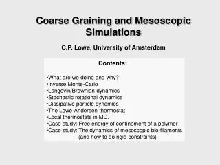
Coarse Graining and Mesoscopic Simulations • Contents: • What are we doing and why? • Inverse Monte-Carlo • Langevin/Brownian dynamics • Stochastic rotational dynamics • Dissipative particle dynamics • The Lowe-Andersen thermostat • Local thermostats in MD. • Case study: Free energy of confinement of a polymer • Case study: The dynamics of mesoscopic bio-filaments • (and how to do rigid constraints) C.P. Lowe, University of Amsterdam
What is coarse graining? Answer: grouping things together and treating them as one object You are already familiar with the concept. Quantum MD Classical MD United atom model n-Alkane
What is mesocopic simulation? Answer: extreme coarse graining to treat things on the mesoscopic scale (The scale ~ 100nm which is huge by atomic standards but where fluctuations are still relevant) 100nm long polymer
N P CO C All-atom model 118 atoms Coarse-grained model 10 sites What are the benefits of coarse graining? Why stop there? Eg. this lipid l lc CPU per time step at least 10 times less (or even better)
N P CO C All-atom model 118 atoms Coarse-grained model 10 sites What are the benefits of coarse graining? Why stop there? Eg. this lipid l lc Maximum time-step Longer time-steps possible
Coarse graining with inverse Monte Carlo Full information (but limited scale) All-atomic model MD simulation Coarse-graining – simplified model RDFs for selected degrees of freedom Effective potentials for selected sites Reconstruct potentials (inverse Monte Carlo) Increase scale Effective potentials Properties on a larger length/time scale
Inverse Monte Carlo direct Model Properties inverse Interaction potential Radial distribution functions • Effective potentials for coarse-grained models from "lower level" simulations • Effective potential = potential used to produce certain characteristics of the real system • Reconstruct effective potential from experimental RDF
Inverse Monte Carlo (A.Lyubartsev and A.Laaksonen, Phys.Rev.A.,52,3730 (1995)) Consider Hamiltonian with pair interaction: Va Make “grid approximation”: | | | | | | | Hamiltonian can be rewritten as: Rcut a=1,…,M WhereVa=V(Rcuta/M)- potential withina-interval, Sa - number of particle’s pairs with distance between them withina-interval Sais an estimator of RDF:
Inverse Monte Carlo In the vicinity of an arbitrary point in the space of Hamiltonians one can write: where with b = 1/kT,
Inverse Monte Carlo Choose trial values Va(0) Direct MC Calculate <Sa>(n) and differences D<Sa>(n) = <Sa >(n) - Sa* Repeat until convergence Solve linear equations system Obtain DVa(n) New potential: Va(n+1) =Va(n) +DVa(n)
Example: vesicle formation Starting from a square plain piece of membrane, 325x325 Å, 3592 lipids: (courtesy of Alexander Lyubartsev ) cut plane
The dispersed phase problem • Many important problems involve one boring species (usually • a solvent) present in abundance and another intersting speices • that is a large molecule or molecular structure. • Examples • Polymer solutions • Colloidal suspensions • Aggregates in solution This is very problematic
The dispersed phase problem Polymers are long molecules consisting of a large number N (up to many millions) of repeating units. For example polyethylene Consider a polymer solution at the overlap concentration (where the polymers roughly occupy all space) L~N1/2b where b is of the order of the monomer size
The dispersed phase problem Volume fraction of momomers Volume fraction of solvent (assuming solvent molecules similar in size to monomers) Number of solvent molecules per polymer So, if N=106, not unreasonable, we need 109 solvent molecules per polymer
Time-scale Configurations change on the time-scale it takes the polymer to diffuse a distance of its own size tD. From the diffusion equation root mean squared displacement D as a function of time t is Experimentally: b (polyethylene) = 5.10-10m b(DNA) = 5.10-8m So for N=106 lp(polyethylene) = 5.10-7m (1/2m) lp(DNA) = 5.10-5m (50m) Use Stokes-Einstein to estimate k=Boltzmann’s constant T=Temperature h=shear viscosity of solvent kT(room temp.)~4.10-14 gcm2/s2 h(water)~0.01 g/cm s So
The dispersed phase problem Configurations change on the time-scale it takes the polymer to diffuse a distance of its own size tD. From the diffusion equation root mean squared displacement D as a function of time t is Coarse graining required Experimentally: b (polyethylene) = 5.10-10m b(DNA) = 5.10-8m So for N=106 lp(polyethylene) = 5.10-7m (1/2m) lp(DNA) = 5.10-5m (50m) Use Stokes-Einstein to estimate k=Boltzmann’s constant T=Temperature h=shear viscosity of solvent kT(room temp.)~4.10-14 gcm2/s2 h(water)~0.01 g/cm s So
v F v’ The ultimate solvent coarse graining Throw it away and reduce the role of the solvent to: 1) Just including the thermal effects (i.e the fluctutations that jiggle the polymer around) 2) Including the thermal and fluid-like like behaviour of the solvent. This will include the “hyrodynamic interactions” between the monomers. Hydrodynamic interactions
The Langevin Equation (fluctuations only) Solve a Langevin equation for the big phase: Force on particle i -gv is the friction force, here the friction coefficient is related to the monomer diffusion coeffiient by D=gkT is a random force with the property is the sum of all other forces Many ways to solve this equation Forbert HA, Chin SA. Phys Rev E 63, 016703 (2001) It is basically a thermostat.
The Andersen thermostat (fluctuations only) Use an Andersen thermostat: A method that satisfies detailed balance (equilibium properties correct) Integrate the equations of motion with a normal velocity Verlet algorithm Then with a probability GDt (G is a “bath” collision probability) set Where qi is a Gaussian random number with zero mean and unit variance. (i.e. take a new velocity component from the correct Maxwellian) Gives a velocity autocorrelation function C(t)=<v(0)v(t)> Identical to the Langevin equation with g/m=G
Andersen vs Langevin Question: Should I ever prefer a Langevin thermostat to an Andersen thermostat? Answer: No. Because Andersen satisfies detailed balance you can use longer time-steps without producing significant errors in the equilibrium properties (who cares that it is not a stochastic differential equation)
Brownian Dynamics (fluctuations and hydrodynamics) Use Brownian/Stokesian dynamics Integrates over the inertial time in the Langevin equation and solve the corresponding Smoluchowski equation (a generalized diffusion equation). As such, only particle positions enter. are “random” displacements that satisfy and is the mobility tensor D.L. Ermak and J.A. McCammon, J. Chem. Phys. 969, 1352 (1978) “Computer simulations of liquids”, M.P. Allen and D.J. Tildesley, (O.U. Press, 1987)
Brownian Dynamics (fluctuations and hydrodynamics) If the mobility tensor is approximated by The algorithm is very simple. This corresponds to neglecting hydrodynamic interactions (HI) Including HI requires the pair terms. A simple approximation based on the Oseen tensor (the flow generated by a point force) is. For a more accurate descrition it is much more difficult but doable, see the work of Brady and co-workers. A. J. Banchio and J. F. Brady J. Chem. Phys. 118, 10323 (2003)
Brownian Dynamics (fluctuations and hydrodynamics) • Limitations: • Computaionally demanding because of long range nature of mobility tensor • Difficult to include boundaries • Fundamentally only works if inertia can be completely neglected So should I just neglect hydrodynamics: NO (hydrodynamics are what make a fluid a fluid)
Simple explicit solvent methods An alternative approach: Keep a solvent but make it as simple as possible (strive for an “ising fluid”). • What makes a fluid: • Conservation of momentum • Isotropy • Gallilean Invariance • The right relative time-scale time it takes momentum to diffuse l time it takes sound to travel l time it takes to diffuse l
Stochastic Rotational dynamics A. Malevanets and R. Kapral, J. Chem. Phys 110, 8605 (1999). Advect collide random grid shift recovers Gallilean invariance
Stochastic Rotational dynamics Collide particles in same cell basically rotates the relative velocity vector where the box centre of mass velocity is with Ncell the number of particles in a given cell. R is the matrix for a rotation about a random axis • Advantages: • Trendy • Computationally simple • Conserves mometum • Conserves energy • Disadvantages • Does not conserve angular momentum • Introduces boxes • Isotropy? • Gallilean invariance jammed in by grid shift • Conserves energy (need a thermostat for non-equilibrium simulations)
Stochastic Rotational dynamics • Equation of state: Ideal gas • Parametrically: exactly the same as all other ideal gas models • must fix • number of particles per cell (cf r) • degree of rotation per collision (cf G) • number of cells traversed before velocity is decorrelated (cf L) • Time-scales • Transport coefficients: theoretical results accurate in the wrong range of parameters. For realistic parameters, must callibrate. • For an analysis see • J.T. Padding abd A.A. Louis, Phys. Rev. Lett. 93, 2201601 (2004)
Dissipative Particle Dynamics part 1: the method First introduced by Koelman and Hoogerbrugge as an “off-lattice lattice gas” method with discrete propagation and collision step. P.J. Hoogerbrugge and J.M.V.A. Koelman, Europhys. Lett. 19, 155 (1992) J.M.V.A. Koelman and P.J. Hoogerbrugge and , Europhys. Lett. 21, 363 (1993) This formulation had no well defined equilibrium state (i.e. corresponded to no known statistical ensemble). This didn’t stop them and others using it though. The formulation usually used now is due to Espanol and Warren. P. Espanol and P.B. Warren, Europhys. Lett. 30, 191, (1995). Particles move according to Newton’s equations of motion:
rij rc Dissipative Particle Dynamics So what are the forces? They are three fold and are each pairwise additive The “conservative” force: where; Is a “repulsion” parameter Is an interaction cut-off range parameter
Dissipative Particle Dynamics What is the Conservative force? Simple: a repulsive potential with the form U(r) aijrc It is “soft” in that, compared to molecular dynamics it does not diverge to infinity at any point (there is no hard core repulsion. rc The “dissipative” force Component of relative velocity along line of centres
Dissipative Particle Dynamics • What is the Dissipative force? • A friction force that dissipates relative momentum • (hence kinetic energy) • A friction force that transports momentum • between particles ? wd rc The random force:
Fluctuation Dissipation 1 To have the correct canonical distribution function (constant NVT) the dissipative (cools the system) and random (heats the system) forces are related: wd rc For historical (convenient?) reasons wd is given the same form as the conservative force The weight functions are related As are the amplitudes
DPD as Soft Particles and a Thermostat Without the random and dissipative force, this would simply be molecular dynamics with a soft repulsive potential. With the dissipative and random forces the system has a canonical distribution, so they act as a thermostat. These two parts of the method are quite separate but the thermostat has a number of nice features. Local Conserves Momentum Gallilean Invariant
Integrating the equations of motion • How to solve the DPD equations of motion is itself something of an issue. • The nice property of molecular dynamics type algorithms (e.g. satisfying • detailed balance) are lost because of the velocity dependent dissipative force. • This is particularly true in the parametrically correct regime • Why is this important? • Any of these algorithms are okay if the time-step is small enough • The longer a time-step you can use, the less computational time your • simulations need • How long a time step can I use? • Beware to check more than that the temperature is correct • The radial distribution function is a more sensitive test. The temperature • can be okay while other equilibrium properties are severely inaccurate. • L-J.Chen, Z-Y Lu, H-J ian, Z-Li, and C-C Sun, J. Chem. Phys. 122, 104907 (2005)
Integrating the equations of motion Euler-type algorithm P. Espanol and P.B. Warren, Europhys. Lett. 30, 191, (1995). And note that, because we are solving a stochastic differential equation (Applies for all the following except the LA thermostat)
Integrating the equations of motion Modified velocity Verlet algorithm R.D. Groot and P.B. Warren, J. Chem. Phys. 107, 4423, (1997). Here l is an adjustable parameter in the range 0-1 • Still widely used • Actually equivalent to the Euler-like scheme
Integrating the equations of motion Self-consistent algorithm: I Pagonabarraga, M.H.J. Hagen and D. Frenkel, Europhys. Lett. 42, 377, (1998). • Updating of velocities is performed iteratively • Satisfies detailed balance (longer time-steps possible) • Computationally more demanding
Which method should I use? 1) It depends on the conservative force (interaction potential). The time step must always be small enough such that the conservative equations of motion adequately conserve total energy. To check this, run the simulation without the thermostat and check total energy. 2) If this limits the time-step the methods that satisfy detailed balance lose their advantage. 3) If not, use the self-consistent or LAT methods. Never Euler or modified Verlet. 4) There are some much better methods that still do not strictly satisfy detailed balance (based on more sophisticated Langevin-type algorithms). W.K. den Otter and J.H.R. Clarke, Europhys. Lett. 53, 426 (2001). T. Shardlowe, SIAM J. Sci. Comput. (USA) 24, 1267 (2003). 5) For a review see P. Nikunen, M. Karttunen and I. Vattulainen, Comp. Phys. Comm. 153, 407 (2003).
Alternatively, change the method • The complications arise because the stochastic differential equation • is difficult to solve without violating detailed balance (see Langevin • vs Andersen thermostats) • In the same spirit let us modify the Andersen scheme such that • Bath collisions exchange relative momentum between pair of particles • by taking a new relative velocity from the Maxwellian distribution for • relative velocities • Impose the new relative velocity in such a way that linear and angular • momentum is conserved. • Following the same arguments as Andersen, detail balance is satisfied Leads to the Lowe-Andersen thermostat
The Lowe-Andersen thermostat Lowe-Andersen thermostat (LAT): C.P.Lowe, Europhys. Lett. 47, 145, (1999). “Bath” collision • Here G is a bath collision frequency (plays a similar role to g/m in DPD) • Bath collisions are processed for all pairs with rij<rc • The current value of the velocity is always used in the bath collision (hence • the lack of an explicit time on the R.H.S.) • The quantity x is a random number uniformly distributed in the range 0-1 • The quantity mij is the reduced mass for particles i and j, mij=mi mj/(mi+mj)
The Lowe-Andersen vs DPD (as a thermostat) • Conserve linear momentum (BOTH) • Conserve angular momentum (BOTH) • Gallilean invariant (BOTH) • Local (BOTH) • Simple integration scheme satisfies detailed balance (LA YES, DPD NO)
The Lowe-Andersen vs DPD (as a thermostat) Disadvantage?: It does not use weight functions wd and wr (or alternatively you could say it uses a hat shaped weight functions) But, no-one has ever shown these are useful or what form they should best take. The form wr=(1-rij/rc) is only used for convenience (work for someone?) They could be introduced using a distance dependent collision probability In the limit of small time-steps LAT and DPD are actually equivalent! E.A.J.F. Peters, Europhys. Lett. 66, 311 (2004). Word of warning: in the LAT, bath collisions must be processed in a random order • Is the DPD thermostat ever better than the Lowe-Andersen thermostat? In simple terms: you can take a longer time-step with LA than with DPD without screwing things up.and there are no disadvantages so…. NO
Can I use these thermostats in normalMD? Yes and in fact they have a number of advantages: 1) Because they are Gallilean invariant they do not see translational motion as an increase in temperature. Nose-Hoover (which is not Gallilean invariant does) T. Soddemann , B. Dünweg and K. Kremer, Phys. Rev. E 68, 046702 (2003) 2) Because they preserve hydrodynamic behavior, even in equilibrium they disturb the dynamics of the system much less than methods that do not (the Andersen thermostat for example)
Can I use these thermostats in normalMD? Example: a well know disadvantage of the Andersen thermostat is that at high thermostating rates diffusion in the system is suppressed (leading to inefficient sampling of phase space) Lowe-Andersen Andersen whereas for the Lowe-Andersen thermostat it is not. E. A. Koopman and C.P. Lowe, J. Chem. Phys. 124, 204103 (2006)
Can I use these thermostats in normalMD? 3) Where is heat actually dissipated? At the boundaries of the system. Because these thermostats are local (whereas Nose-Hoover is global) one can enforce local heat dissipation. Carbon nanotube modelled by “frozen” carbon structure Heat exchange of diffusants with the nanotube modelled by local thermostating during diffusant-microtubule interactions S. Jakobtorweihen,M. G. Verbeek, C. P. Lowe, F. J. Keil, and B. Smit Phys. Rev. Lett. 95, 044501 (2005)
DPD Summary • The dissipative and random forces combine to act as a thermostat • (Fullfilling the same function as Nose-Hoover or Andersen thermostats • in MD) • As a thermostat it has a number of advantages over some commonly • used MD thermostats • The conservative force corresponds to a simple soft repulsive harmonic • potential between particles, but in principle it could be anything • (The DPD thermostat can also be used in MD • T. Soddemann, B. Dunweg and K. Kremer, Phys. Rev. E68, 046702 (2003) ) • The equations of motion are awkward to integrate accurately with • large time-steps. Chose your algorithm and test it with care. • The Lowe-Andersen thermostat has the same features as the DPD • thermostat but is computationally more efficient as it allows longer • time-steps.
Dissipative particle dynamics part 2: why this form for the conservative force? In principle the conservative force can be anything you like, what are the reasons for this choice? Some common statements; “It is the effective interaction between blobs of fluid” No it isn’t, at least not unless you are very careful about what you mean by effective. “A soft potential that allows longer time-steps” Maybe, but relative to what? Factually: it is not a Lennard-Jones (or molecular-like) potential. It is the simplest soft potential with a force that vanishes at some distance rc As with any soft potential it has a simple equation of state in the fluid regime and at high densities.
The equation of state of a DPD Fluid For a single component fluid with pairwise additive spherically symmetric interparticle potentails the pressure P in terms of the radial distribution function g(r) is where r is the density. For a soft potential with range rc at high densities, r>>3/(4prc3) g(r)~1 so g(r) real fluid g(r) DPD fluid Where a is a constant. For DPD a=.101aijrc4 • Note though that : • If r is too high or kT too low the DPD fluid will freeze • making the method useless. • And a/kT is not the the true second Virial coefficient • so this does not hold at low densities EoS
Mapping a DPD Fluid to a real fluid R.D. Groot and P.B. Warren, J. Chem. Phys. 107, 4423, (1997). Match the dimensionless compressibility k for a DPD fluid to that ofreal fluid For a (high density) DPD fluid, from the equation of state For water k-1~16 so in DPD aij=75kT/rrc4 Once the density is fixed, this fixes the repulsion parameter. You can use a similar procedure to map the dimensionless compressibility of other fluids.
P FTh P0 x What’s right and what’s wrong By setting the dimensionless compressibility correctly we will get the correct thermodynamic driving forces FThfor small pressure gradients (the chemical potential gradient is also correct) Technically, we reproduce the structure factor at long wavelengths correctly. But, other things are completely wrong, eg the compressibility factor P/rkT And this assumes on DPD particle is one water molecule. If it represents n water molecules the r(real)=nr(model) so aij must be naij(n=1). That is the repulsion parameter is scaled with n and if n>1 the fluid freezes. R.D. Groot and K.L. Rabone, Biophys. J. 81, 725 (2001).