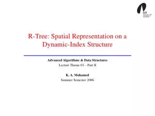
R-Tree: Spatial Representation on a Dynamic-Index Structure
460 likes | 679 Views
R-Tree: Spatial Representation on a Dynamic-Index Structure. Advanced Algorithms & Data Structures Lecture Theme 03 – Part II K. A. Mohamed Summer Semester 2006. Overview. Representing and handling spatial data The R-Tree indexing approach, style and structure Properties and notions

R-Tree: Spatial Representation on a Dynamic-Index Structure
E N D
Presentation Transcript
R-Tree: Spatial Representation on a Dynamic-Index Structure Advanced Algorithms & Data Structures Lecture Theme 03 – Part II K. A. Mohamed Summer Semester 2006
Overview • Representing and handling spatial data • The R-Tree indexing approach, style and structure • Properties and notions • Searching and inserting index Entry-records • Deleting and updating • Performance analyses • Node splitting algorithms • Derivatives of the R-Trees • Applications
Deletion • Current index entry-records are removed from the leaves. • Nodes that underflow are condensed, and its contents redistributed appropriately throughout the tree. • A condense propagation may cause the tree to shorten in height. The main Delete routine • Let E = (I, tuple-identifier) be a current entry to be removed. • Let T be the root of the R-Tree. • [Del_1]Find the leafL starting from T that contains E. • [Del_2]RemoveE from L, and condense ‘underflow’ nodes. • [Del_3]Propagate MBR changes upwards. • [Del_4]Shortentree if T contains only 1 entry after condense propagation.
Deletion – Find Leaf [Del_1]Find the leafL starting from T that contains E. Algorithm: FindLeaf (E, N) Inputs: (i) Entry E = (I, tuple-identifier), (ii) A valid R-Tree node N. Output: The leaf L containing E. • IfN is leaf Then • IfN contains EThenReturnN • ElseReturn NULL • Else • Let FS be the set of current entries in N. • For each F = (I, child-pointer) FS where F.I overlaps E.IDo • Set L = FindLeaf (E, F.child-pointer) • IfL is not NULL ThenReturnL • NextF • Return NULL • End If
Deletion – Remove and Adjust [Del_2]RemoveE from L, and condense ‘underflow’ nodes. [Del_3]Propagate MBR changes upwards. • Notion (i): Ascend from leaf L to root T while adjusting covering rectangles MBR. • Notion (ii): If after removing the entry E in L and the number of entries in L becomes fewer than m, then the node L has to be eliminated and its remaining contents relocated.
Deletion – Remove and Adjust • Propagate these notions upwards by invoking CondenseTree (N, QS), where N is an R-Tree node whose entries have been modified, and QS is the set of eliminated nodes. • Start the propagation by setting N = L, and QS = . • Re-insert the entries from the eliminated nodes in QS back into the tree. • Entries from eliminated leaf nodes are re-inserted as new entries using the Insert routine discussed earlier. • Entries from higher-level nodes must be placed higher in the tree so that leaves of their dependent subtrees will be on the same level as the leaves on the main tree.
@ r6 @ r7 @ r2 r0 r2 r3 r4 r1 r6 r5 @ r0 @ r3 @ r4 @ r5 @ r1 a k i f c d g b j l h m e n Deletion – Propagating Node Condensation Example: R-Tree settings: M = 4, m = 2. • Delete the index entry-record h. • Delete the index entry-record b. Note: a.I will form smallest MBR with r4.
Deletion – Condense Tree (I) Algorithm: CondenseTree (N, QS) Inputs: (i) A node N whose entries have been modified, (ii) A set of eliminated nodes QS. • IfN is NOT the root Then • Let PN be the parent node of N. • Let EN = (I_N, child-pointer_N) in PN. • IfN.entries < mThen • Delete EN from PN • Add N to QS • Else • Adjust I_N so that it tightly encloses all entry regions in N. • End If • CondenseTree (PN, QS)
Deletion – Condense Tree (II) • Else If N is root AND QS is NOT Then • For each QQSDo • For each EQDo • IfQ is leaf ThenInsert (E) • ElseInsert (E) as a node entry at the same node level as Q • End If • NextE • NextQ • End If [Del_4]Shortentree if T contains only 1 entry after condense propagation.
Deletion – Summary Why ‘re-insert’ orphaned entries? • Alternatively, like the delete routine in B-Tree (Rosenberg & Snyder, 1981), an ‘underflow’ node can be merged with whichever adjacent sibling that will have its area increased the least, or its entries re-distributed among sibling nodes. • Both methods can cause the nodes to split. • Eventually all changes need to be propagated upwards, anyway.
Deletion – Summary Re-insertion accomplishes the same thing, and: • It is simpler to implement (and at comparable efficiency). • It incrementally refines the spatial structure of the tree. • It prevents gradual deterioration if each entry was located permanently under the same parent node.
Updating Changes in Spatial Objects • When a spatial object in a leaf entryE (pointed to by E.tuple-identifier) changes in size, its MBR contained in E.I must reflect this change. • BUT, instead of simply updating the value for E.I, we should: • Delete E from the tree. • Create a new entry E’ for the affected change in the spatial object. • Insert E’ into the tree using the Insert() routine.
Updating Changes in Spatial Objects Why? Because… • Rather than percolating a stagnant change from the leaf level upwards, we let E’ find its way down the tree to the most appropriate location. • See notion on ‘optimal placement emphasis’. Is it more expensive? • Case 1: Percolate new change from Leaf. • Case 2: Delete and re-insert new change from Root.
Performance with respect to Parameter m • A high value of m, nearer to M, is useful when the underlying database is mostly used for search inquiries with very few updates. • The height of the tree will be kept to a minimum. • High search performance is maintained. • However, the risk of overflow and underflow is also high. • A small value of m is good when frequent updates and modifications of the underlying database is required. • The nodes are less dense. • Maintenance is less costly.
Overview • Representing and handling spatial data • The R-Tree indexing approach, style and structure • Properties and notions • Searching and inserting index Entry-records • Deleting and updating • Performance analyses • Node splitting algorithms • Derivatives of the R-Trees • Applications
Node Splitting • Happens when the node-overflow condition is triggered. • We need to divide the M+1 entries between N and N’ (equally). • Notion: The consolidated entries in N and N’ must make it as unlikely as possible that both nodes will need to be examined on subsequent searches. • Already implemented and used in ChooseLeaf() in the Insert() routine. • Objective: To minimise the resulting MBRs of N and N’ after consolidation. • Supplement: The smaller the covering regions, the smaller the possibility that they overlap with other MBRs.
c c a a b b d d Node Splitting Bad split Good split
Node Splitting – Naïve • The greedy and straight forward algorithm to find the minimum area node split is by brute force. • Generate all possible groupings and take the best one. • Total possibilities (for M entries, 2 nodes): • Advantage: • Disadvantage:
@ r6 r2 r5 @ r2 @ r5 r0 r3 r1 r4 I(a) = {[30, 105], [0, 80]} I(b) = {[0, 220], [125, 280]} I(c) = {[60, 80], [370, 390]} I(d) = {[270, 300], [190, 215]} I(e) = {[210, 315], [260, 350]} I(f) = {[320, 360], [245, 285]} I(g) = {[195, 270], [415, 480]} I(h) = {[360, 430], [115, 205]} I(i) = {[700, 815], [500, 560]} @ r0 @ r3 @ r1 @ r4 a b c g d e f h i Optimised Example: Map of Freiburg
Node Splitting – Quadratic Cost • The Quadratic-Cost algorithm attempts to find a small-area split, but cannot guarantee the smallest possible area. • Notion (i): Pick 2 seed-entries that are most distant from each other, and put them in 2 separate nodes N and N’. • Notion (ii): The remaining entries are picked and then assigned to either groups one at a time. • Notion (iia): Manner of picking next entry to insert: Outer boundary to the inner circle. • Notion (iib): Manner of assigning: Add to node whose MBR will have to be enlarged the least (resolve ties by picking node whose MBR is smaller).
Node Splitting – Quadratic Cost: Pick Seeds Algorithm: PickSeeds (ES) Input: ES : A set of M+1 entries. Outputs: 2 entries Ei and Ej that are furthest apart. • Let ES = {E0, E1, …, EM} • For each Ei from E0 to EM-1Do • For each Ej from Ei to EMDo • Compose a region R that includes Ei.I and Ej.I • Calculate ∂ = area(R) – area(Ei.I) – area(Ej.I) • NextEj • NextEi • ReturnEi and Ej with the largest ∂
Node Splitting – Quadratic Cost: Pick Next Algorithm: PickNext (ES, N, N’) Inputs: ES : A set of entries not yet in N or N’. Output: The next entry E to be considered for assignment. • Let ES = {E0, E1, …, Ek} • For each E from E0 to EkDo • Calculate ∂N = area increase req. in the MBR of N to include E.I • Calculate ∂N’ = area increase req. in the MBR of N’ to include E.I • NextE • ReturnE with the maximum difference between ∂N and ∂N’
Node Splitting – Quadratic Split Algorithm Algorithm: QuadraticSplit (ES, N, N’) Inputs: ES : A set of entries ES to be split into N and N’. • Let {EA, EB} = PickSeeds (ES), be the first entries in N and N’ respectively • Let ES’ = ES – {EA, EB}. • WhileES’ still has entries to be assigned Do • If either N or N’ has m entries Then • Add all of ES’ into either N or N’ that has fewer than m entries • Else • Let E = PickNext (ES’, N, N’) • Add E into either N or N’ following Notion (iib) • End If • Update ES’ • Loop
Node Splitting – Linear Split • The Linear-Split algorithm is the same as the Quadratic-Split algorithm, but • Uses LinearPickSeeds() instead of PickSeeds(). • Randomly chooses next entry for assignment instead of using PickNext(). • Notion: Examine each Interval [ka, kb] spanning each dimension for every Entry, and select 2 Entries that are most distant from each other.
Node Splitting – Linear Pick Seeds Algorithm: LinearPickSeeds (ES) Input: ES : A set of M+1 entries. Outputs: 2 entries Ei and Ej that are deemed furthest apart. • Let ES = {E0, E1, …, EM} • For each dimension d from 1 to nDo • Let Ei and Ej be the 2 entries farthest away from each other in dimension d, such that Ei.I = [dai, dbi] has the highest lower-bounddai and Ej.I = [daj, dbj] has the lowest upper-bounddaj • Calculate wid_d = daj – dai • Normalise wid_d to the width of the entire set on this d • Nextd • ReturnEi and Ej with the largest wid_d
Node Splitting – Linear Pick Seeds d = 1 d = 0
Overview • Representing and handling spatial data • The R-Tree indexing approach, style and structure • Properties and notions • Searching and inserting index Entry-records • Deleting and updating • Performance analyses • Node splitting algorithms • Naïve-Split • Quadratic-Split • Linear-Split • Derivatives of the R-Trees • Applications
Derivatives of the R-Tree • Concepts and index-structure of the original R-Tree remains the same. • Derivatives of the R-Trees emphasise on improvements on optimisation methods topack rectangles based on other imposed constraints. • 2 main constraint-issues addressed in the literature: • Coverage: Total area of all the MBRs of all leaf nodes. • Overlap: Total area contained within 2 or more leaf MBRs. • For efficient R-Tree searching: Bothcoverage and overlap must be minimised. • Overlap condition is more critical than coverage to achieve maximum efficiency in searching. • However, it is difficult to control overlaps during dynamic splits.
c Q P b a d Derivative I: R+ Tree Notion: Avoid overlaps among MBRs at the expense of space. • Rectangles are decomposed into smaller sub-rectangles. • A leaf-MBR L.I that overlaps other MBRs is broken into several non-overlapping rectangles (whose union makes up L.I). • All pointers of the sub-rectangles point to the same object L.tuple-identifier. • Sub-rectangles chosen so that no MBR at any level needs to be enlarged.
b P a Q c Derivative II: R*-Tree Notion: Avoid overlaps among MBRs, while optimising space. • Similar constraints as in the R+ Tree, but differ in choosing the path of least resistance when inserting new index-records. • Favours smallest variation in margin length, in addition to choosing the smallest encompassing area. Example: Suppose Area(P) ≈ Area(Q)
Derivative III: X-Tree Notion: (A variant specifically designed for dealing with high-dimensional space) Dynamically organise the tree such that portions of the data which would produce high overlap are organised linearly in extended supernodes. • Employs the concept of weighted overlap, measured by the number of rectangles within an overlapping region.
Derivative III: X-Tree • The X-Tree uses extended variable-size supernodes with αM entries, α> 1. • Supernodes are used to avoid splits with high overlap values. • Studies show that overlaps increase with dimension. • Supernodes are created during insertion only if there is no possibility to avoid high overlaps. Berchtold, Keim and Kriegel. (1996)
Overview • Representing and handling spatial data • The R-Tree indexing approach, style and structure • Properties and notions • Searching and inserting index Entry-records • Deleting and updating • Performance analyses • Node splitting algorithms • Derivatives of the R-Trees • R+ Tree • R*-Tree • X-Tree • Applications
Interactive Graphic-Objects (IGO) on 2D Screen Scene Spatial-objects Screen-surface Consider • Placing (spatial) 3D-graphic-objects in a scene. • Screen display is 2D. • Objects have depth-perception. Interactions • Clicking (2D Point) returns ONE correctly selected object. R-Tree Structure • Assumptions? • Support dimension? • Augment information? Deeper in the scene Closer to the screen-surface
IGO: Assumptions • That the scene is static; i.e. camera view on screen-surface don’t change. • That we are dealing only with one snapshot at time ts. • That the (spatial) objects are static at ts; following (ii). • That 3D objects and scene are flattened for 2D display on screen-surface. • That depth-perception is realised on size of objects; they appear relatively smaller when deeper in the scene, and relatively larger otherwise. • That objectscloser to the screen-surface are always drawn on top ofobjects that are deeper in the scene. • That within the MBR of the objects, we can tell whether or not the object itself has been clicked on (e.g. via Quad-trees).
IGO: Problem Formulation Objective: Clicking must return the correct object viewed on 2D screen. • Case 1: Non-overlapping objects. Straight forward • Case 2: Overlapping objects. • Notion (i): Perform a stabbing query – use point p as query point and return all leaf entries stabbed by p. • Notion (ii): Return the ONE object closest to the screen-surface. Additional Requirements • Augment ‘layer’ values in the R-Tree nodes; such that objects deeper in the scene would have lower ‘layer’ values than objects closer to the screen surface. • Modify entry EN = (I, *pointer, vl, vh), where vl is the lowest ‘layer’ value at the subtree of node N, and vh is the highest ‘layer’ value.
h b d e a c g f IGO: Structure – Spatial View Level Order: Deepest in scene (0), closest to screen-surface (7). I(a) = {[76, 234], [160, 402]} I(b) = {[93, 168], [243, 344]} I(c) = {[147, 290], [340, 460]} I(d) = {[202, 264], [294, 398]} I(e) = {[307, 416], [299, 444]} I(f) = {[234, 439], [245, 507]} I(g) = {[342, 700], [100, 500]} I(h) = {[440, 613], [12, 338]}
@ r6 @ r5 @ r2 @ r0 @ r1 @ r3 @ r4 IGO: Structure – Tree View
IGO: Search Strategy • Algorithm: IGOSearch (N, p) • Inputs: (i) A node N in the R-Tree, (ii) The clicked point p. • Output: The leaf entry EL stabbed by p which is on the top-most layer. • IfN is Leaf Then • Let ES be the set of entries in N whose spatial objects are stabbed by p. • IfES = ThenReturn NULL • ElseReturnEL= (I, child-pointer, vl, vh) ES whose vh is the highest
IGO: Search Strategy • Else • Let ES be the set of child-node entries in N whose I’s containp. • Arrange ES in decreasing order of vh. • For each EN = (IN, child-pointer_N, vlN, vhN) ESDo • Store EL = IGOSearch (child-pointer_N, p) • NextEN • ReturnEL= (I, child-pointer, vl, vh) ES whose vh is the highest • End If
Summary & Conclusions • The R-Tree has similar features and properties to the B-Tree. • They remain height balanced while maintaining adjustable rectangles that ignore ‘dead spaces’. • The structure and composition in R-Trees are dynamically driven by the spatial objects they represent. • The spatial objects stored at the leaf-level are considered ‘atomic’, as far as the search is concerned; i.e. they are not further decomposed into pictorial primitives. • The performance of the R-Tree is based on the optimality of packing lower level rectangles in higher level nodes. • Splitting nodes contribute to localimprovement of rectangular arrangements. • Condensing nodes contribute to globalrefinement of rectangular arrangements.
References • A. Guttman. R-trees: A dynamic index structure for spatial searching. In Proceedings of the International Conference of Management of Data (ACM SIGMOD), pages 47-57. ACM Press, 1984. • N. Roussopoulos, C. Faloutsos, and T. Sellis. An efficient pictorial database system for PSQL. In IEEE Transactions on Software Engineering, 14(5):639-650. IEEE Press, 1988. • N. Beckmann, H.-P. Kriegel, R. Schneider, and B. Seeger. The R*-tree: an efficient and robust access method for points and rectangles. In Proceedings of the International Conference of Management of Data (ACM SIGMOD), pages 322-331. ACM Press, 1990. • S. Berchtold, D. A. Keim, and H.-P. Kriegel. The X-tree: An index structure for high-dimensional data. In Proceedings of the 22nd International Conference on Very Large Databases, pages 28-39. Morgan Kaufmann Publishers, 1996.