Data Visualization
Data Visualization. The commonality between science and art is in trying to see profoundly - to develop strategies of seeing and showing Edward Tufte.

Data Visualization
E N D
Presentation Transcript
Data Visualization The commonality between science and art is in trying to see profoundly - to develop strategies of seeing and showing Edward Tufte
A graphical representation of Napoleon Bonaparte's invasion of and subsequent retreat from Russia during 1812. The graph shows the size of the army, its location and the direction of its movement. The temperature during the retreat is drawn at the bottom of figure, which was drawn by Charles Joseph Minard in 1861 and is generally considered to be one of the finest graphs ever produced.
R • R is a free software environment for statistical computing and graphics • It runs on a wide variety of platforms
ggplot An implementation of the grammar of graphics in R The grammar describes the structure of a graphic A graphic is mapping from data to visual properties of geometric shapes
Process of graphing A series of independent steps to produce a holistic visual
Geoms • Graphical objects • Point • Path • Polygon • Interval • Rectangle • Schema • Box plot
Statistical transformation Changes the data Should make it more meaningful Counts Smoothing Aggregation
Aesthetics • Continuous • Size • Rotation • Thickness • Categorical • Shape • Color • Position • Coordinate system
Coordinates • Polar • Pie chart • Hierarchical • Mosaic
Facetting What variables should make up the rows and columns
Components of a graphic • Default settings • Statistics + geoms • Data + aesthetic mappings • Scales • Coordinate system • Facets
ggplot2 • Implements grammar of graphics in R • Documentation • Web • http://had.co.nz/ggplot2/ • Book • ggplot2: Elegant Graphics for Data Analysis
ggplot2 install.packages("ggplot2") library(diamonds, package="ggplot2") • 54,000 observations • 4 measures of quality • 5 physical measurements
Select sample # For demonstration purposes, it is quicker to plot a small number of points than the entire set set.seed(1410) # Make the sample reproducible dsmall <- diamonds[sample(nrow(diamonds), 100), ] # select 100
Basic plotting ggplot(dsmall,aes(x=carat,y=price))+ geom_point()
Transforming ggplot(dsmall,aes(x=log(carat),y=log(price))) + geom_point()
Aesthetics ggplot(dsmall,aes(x=carat,y=price,color=color)) + geom_point() ggplot(dsmall,aes(x=carat,y=price,shape=cut)) + geom_point()
Geom Fit a smoother to the data Shows standard error ggplot(dsmall,aes(x=carat,y=price)) + geom_smooth()
Geom Multiple geoms ggplot(dsmall,aes(x=carat,y=price)) + geom_smooth() + geom_point()
Geom Histogram ggplot(dsmall,aes(x=carat)) + geom_histogram()
Geom Density plot ggplot(dsmall,aes(x=carat,color=color)) + geom_density()
Geom • Bar chart • The discrete analog of a histogram ggplot(dsmall,aes(x=color)) + geom_bar()
MySQL & R install.packages("RJDBC") library("RJDBC") drv <- JDBC("com.mysql.jdbc.Driver", "SSD250/Library/Java/Extensions/mysql-connector-java-3.1.18-bin.jar") # connect to the database con <- dbConnect(drv, "jdbc:mysql://wallaby.terry.uga.edu:3306/ClassicModels", user="student", password="student") dbListTables(con)
MySQL & R # Load table d <- dbReadTable(con, "Products") # Plot product lines # Internal fill color is red ggplot(d,aes(x=productLine)) + geom_histogram(fill='red')
MySQL & R # Load table d <- dbReadTable(con, "Payments") # Boxplot of amounts paid ggplot(d,aes(factor(0),amount)) + geom_boxplot(outlier.colour='red') + xlab("") + ylab("Check")
MySQL & R # Load table d <- dbReadTable(con, "Products") # Plot product lines ggfluctuation(table(d$productLine,d$productScale))
MySQL & R # Load table d <- dbReadTable(con, "Products") # Plot product lines ggfluctuation(table(d$productLine,d$productScale),type="color")
MySQL & R # Query table q <- dbGetQuery(con,"SELECTMONTH(orderDate) AS orderMonth, sum((quantityOrdered*priceEach)) AS orderValue FROM Orders, OrderDetails WHERE Orders.orderNumber = OrderDetails.orderNumber GROUP BY orderMonth") # Plot data ggplot(q,aes(x=orderMonth,y=orderValue)) + geom_point(color='green')
MySQL & R # Add some labels to a line graph ggplot(q,aes(x=orderMonth,y=orderValue)) + geom_line(color='blue') + xlab('Month') + ylab('Value of orders ($)')
MySQL & R # Disaggregate by month q <- dbGetQuery(con,"SELECTMONTH(orderDate) AS orderMonth, YEAR(orderDate) AS orderYear, sum((quantityOrdered*priceEach)) AS ordersValue FROM Orders, OrderDetails WHERE Orders.orderNumber = OrderDetails.orderNumber GROUP BY orderYear, orderMonth") ggplot(q,aes(x=orderMonth,y=ordersValue)) + geom_point()
Key points • You can easily visualize the results of SQL queries using R • ggplot is based on a grammar of graphics • Very powerful and logical • The combination of MySQL and R provides a sound platform for data reporting