Download
1 / 23
230 likes | 436 Views
Steady State Analysis of an Open Economy General Equilibrium Model for Brazil. Mirta Noemí Sataka Bugarin (Eco/UnB) Roberto de Goes Ellery Jr(Eco/UnB) Victor Gomes Silva(UCB/UnB) Marcelo Kfoury Muinhos (DEPEP/Bacen). Objective.

E N D
Steady State Analysis of an Open Economy General Equilibrium Model for Brazil Mirta Noemí Sataka Bugarin (Eco/UnB) Roberto de Goes Ellery Jr(Eco/UnB) Victor Gomes Silva(UCB/UnB) Marcelo Kfoury Muinhos (DEPEP/Bacen)
Objective • Numerical characterization of steady state equilibrium for an open general equilibrium model, parameterized for the Brazilian economy. • Quantify how monetary and fiscal policies affect the model economy long-run equilibrium.
Main feature of the Model economy • Transaction technology, Ljungqvist and Sargent (2001), is introduced in order to obtain monetary equilibrium. • Production included in the model economy. • Small open economy.
Model set up • Households
s.t. (2) 1 = lt + ht + s(ct,,mt+1/Pt) In particular transaction technology takes the form: s(ct, mt+1/Pt) = ct [1/(1+ mt+1/Pt)]. Given law law of motion for capital formation: as well as initial conditions (k0, m0, b0) > 0, assuming:
Productive sector Competitive firms, competitive factor’s market and constant return to scale technology:
Government Tax revenue: Seignorage: Debt financing:
Government (cont.) Public expenses: Assuming PPP holds, e($/R$)=P*/P. Government budget constraint, all t ≥ 0:
Allocation of resources Total production allocation: Balance of Payment:
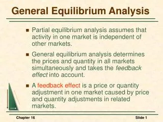
Definition: competitive general equilibrium Sequences of , such that given (i) exogenous sequences for and policy parameters, i.e. (iii) the law of motion for assets ,
Strategy to compute GCE • Formulate DPP. • Derive Euler equations (set of necessary conditions) using differentiability property of Value Function. • Obtain algebraic steady state solution for endogenous variables. • Calibrate model economy with parameter values derived from observed economy. • Compute numerical solution.
Fig. 1 Aggregate Debt Output Ratios at Alternative Steady States
Fig 2. Operational Deficit Output Ratio at Alternative Steady States
Fig. 3 Domestic Debt Output Ratio at Alternative Steady States
Fig. 4 Seignorage Revenue, Operational Deficit and Aggregate Debt as Ratios to Aggregate Output at Alternative Steady States
Fig. 8 Tax rate, Interest rate and Operational Debt – Output ratio.
Fig 9. Tax rate, Interest rate and Domestic debt – output ratio
Conclusion 1. Under adopted parameterization, an aggregate D/Y ratio of 0.3387 is attained at the steady state equilibrium. This equilibrium is supported by a tax share on aggregate output of 17.87%, given a tax rate of 20% and a participation of government expenses of about 17% in aggregate output. 2. Simulation of alternative steady states has shown a clear trade off between higher interest rates (low inflation rates) and higher debt output ratios in the long run. Extension Extensions to analyze short run dynamics of the system are under development. Impulse responses to demand shocks (via monetary policy interventions) and to supply shocks (via exogenous productivity shocks) can be introduced to compute a rational expectation competitive equilibrium.