Download

1 / 18
180 likes | 211 Views
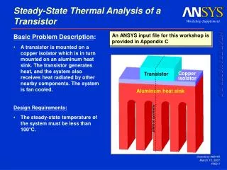
Analyze heat transfer characteristics by comparing surface temperatures & heat flux distribution in plastic and aluminum pump housing models.

E N D
Workshop 6.1 Steady State Thermal Analysis
Workshop 6.1 - Goals • In this workshop we will analyze the pump housing shown below for its heat transfer characteristics. • Specifically a plastic and an aluminum version of the housing will be analyzed using the same boundary conditions. • Our goal is to compare the exposed surface temperatures for each configuration and to investigate the distribution of heat flux in the part. August 26, 2005 Inventory #002266 WS6.1-2
Workshop 6.1 - Assumptions Assumptions: • The pump housing is mounted to a pump which is held at a constant 60 deg. C. We assume the mating face on the pump is also held at this temperature. • The interior surfaces of the pump are held at a constant temperature of 90 deg. C by the fluid. • The exterior surfaces are modeled using a simplified convection correlation for stagnant air at 20 deg. C. August 26, 2005 Inventory #002266 WS6.1-3
Workshop 6.1 - Start Page • From the launcher start Simulation. • Choose “Geometry > From File . . . “ and browse to the file “Pump_housing.x_t”. • When DS starts, close the Template menu by clicking the ‘X’ in the corner of the window. August 26, 2005 Inventory #002266 WS6.1-4
4 Workshop 6.1 - Preprocessing • Change the part material to “Polyethylene”: • Highlight “Part1” • In the Detail window “Material” field “Import . . .” • “Choose” material “Polyethylene”. 1 2 3 • Set the working units to (m, kg, N, C, s, V, A) “Units” menu choose August 26, 2005 Inventory #002266 WS6.1-5
Workshop 6.1 - Environment • Highlight the Environment branch. Select the interior (13) surfaces of the pump housing (hint: use Extend Selection feature). • “RMB > Insert > Temperature”. • Set “Magnitude” field to 90 C. 5 6 7 August 26, 2005 Inventory #002266 WS6.1-6
. . . Workshop 6.1 - Environment • Select the mating surface (1) of the pump housing. • “RMB > Insert > Temperature”. • Set “Magnitude” field to 60 C. 8 9 10 August 26, 2005 Inventory #002266 WS6.1-7
. . . Workshop 6.1 - Environment • Select the exterior (32) surfaces of the pump housing (hint: use extend to limits). • “RMB > Insert > Convection”. 11 12 August 26, 2005 Inventory #002266 WS6.1-8
14 15 . . . Workshop 6.1 - Environment • In the Details change the “Type” field from “Constant” to “Temperature-Dependent”. • “Import” the correlation “Stagnant Air – Simplified Case”, if necessary. • Set the “Ambient Temperature” field to 20 deg. C. 13 August 26, 2005 Inventory #002266 WS6.1-9
16 17 Workshop 6.1 - Solution • Add temperature and total heat flux results. • Highlight the Solution branch. • “RMB > Insert > Thermal > Temperature” • Repeat the above steps to add “Total Heat Flux”. August 26, 2005 Inventory #002266 WS6.1-10
18 19 20 21 Workshop 6.1 – Duplicate Model • Before solving we will duplicate the model and specify a different material for the pump housing. This will allow us to compare the responses for each. • Highlight the “Model” branch. • “RMB > Duplicate”. • From the new branch “Model2” highlight “Part1” • In the detail window “Import” the material “Aluminum Alloy”. August 26, 2005 Inventory #002266 WS6.1-11
22 Workshop 6.1 - Solution • Highlight the “Project” branch in the tree and solve. • Note: by issuing a solve from the Project branch both Model branches will be solved. If single solutions are desired highlight only the branch to be solved before beginning the solve. August 26, 2005 Inventory #002266 WS6.1-12
Workshop 6.1 - Postprocessing • When the solutions are complete, inspect the temperature plots and compare. It can be seen quickly that the choice of material in this case has a significant effect. Polyethylene Aluminum August 26, 2005 Inventory #002266 WS6.1-13
. . . Workshop 6.1 - Postprocessing • A similar comparison of the heat flux in each model points up differences. Here a vector heat flux plot is shown in wireframe mode. Note how much of the energy in the aluminum model is returned via the mating face. Aluminum Polyethylene August 26, 2005 Inventory #002266 WS6.1-14
. . . Workshop 6.1 - Postprocessing • To better view the exterior surface temperatures we will employ scoping as in previous workshops. • Select the outside (32) surfaces of the pump housing (use extend to limits). • “RMB > Insert > Thermal > Temperature” (note the scope of the new result now indicates “32 Faces” rather than “All Bodies” • Using RMB, copy/paste the new result into Model 2 Solution branch. Notice the scope of the result remains in tact. • Solve from the Project branch. 23 24 August 26, 2005 Inventory #002266 WS6.1-15
. . . Workshop 6.1 - Postprocessing • The 2 new plots now display outside temperatures for both models. Notice the contours are not affected by interior temperatures as were the previous plots. Polyethylene Aluminum August 26, 2005 Inventory #002266 WS6.1-16
Workshop 6.1 - Reporting • If time permits, create figures to include in a report and generate the report. August 26, 2005 Inventory #002266 WS6.1-17