Chapter 5 Single-Phase System

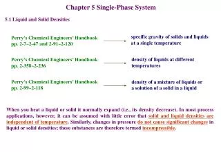
1. Chapter 5 Single-Phase System 5.1 Liquid and Solid Densities specific gravity of solids and liquids at a single temperature Perry’s Chemical Engineers’ Handbook pp. 2-7~2-47 and 2-91~2-120 density of liquids at different temperatures Perry’s Chemical Engineers’ Handbook pp. 2-358~2-236 Perry’s Chemical Engineers’ Handbook pp. 2-99~2-118 density of a mixture of liquids or a solution of a solid in a liquid When you heat a liquid or solid it normally expand (i.e., its density decrease). In most process applications, however, it can be assumed with little error that solid and liquid densities are independent of temperature. Similarly, changes in pressure do not cause significant changes in liquid or solid densities; these substances are therefore termed incompressible.

2. In the absence of data, the density of a mixture of n liquids (A1, A2,…., An) can be estimated from the component mass fractions [xi] and pure-component densities [i] in two ways. Assuming volume additivity and recognizing that component masses are always additive specific volume Averaging the pure-component densities, weighting each one by the mass fraction of the component Figure 5.1-1 at 20C provides a slightly better estimate for methanol and water mixtures of liquid species with similar molecular structures (e.g., all straight-chain hydrocarbons of nearly equal molecular weight, such as n- pentane, n-hexane, and n-heptane) provides a much better estimate for sulfuric and water no general rules Test Yourself p. 190

3. Example 5.1-1 Determine the density in g/cm3 of a 50 wt% aqueous solution of H2SO4 at 20C, both by (1) looking up a tabulated value and (2) assuming volume additivity of the solution components. Solution 1. Look it up Perry’s Chemical Engineers’ Handbook pp. 2-107 and 2-108 2. Estimate it

4. 5.2 Ideal Gas Looking up a density or specific volume at one temperature and pressure and using it at another temperature and pressure usually works well for a solid or a liquid, but not at all for a gas. An expression is needed for gases that relates specific volume to temperature and pressure, so that if any two of these quantities are known the third can be calculated. An equation of state relates the molar quantity and volume of a gas to temperature and pressure. The simplest and most widely used of these relationships is the ideal gas equation of state (PV=nRT), which, while approximate, is adequate for many engineering calculations involving gases at low pressures. However, some gases deviate from ideal behavior at nearly all conditions and all gases deviate substantially at certain conditions (notably at high pressures and/or low temperatures). In such case it is necessary to use more complex equations of state for PVT calculations.

5. 5.2a The Ideal Gas Equation of State The ideal gas equation of state can be derived from the kinetic theory of gases by assuming that gas molecules have a negligible volume, exert no forces on one another, and collide elastically with the walls of their container. P = absolute pressure of a gas = volume (volumetric flow rate) of the gas = number of moles (molar flow rate) of the gas R = the gas constant, whose values depends on the units of P, V, n, and T T = absolute temperature of the gas specific molar volume of the gas A gas whose PVT behavior is well represented by this equation is said to behave as an ideal gas or a perfect gas. The use of this equation does not require a knowledge of the gas species: 1 mol of an ideal gas at 0C and 1 atm occupies 22.415 liters, whether the gas is argon, nitrogen, a mixture of propane and air, or any other single species or mixture of gases.

6. The ideal gas equation of state is an approximation. It works well under some conditions – generally speaking, at temperatures above 0C and pressures below about 1 atm – but at other conditions its use may lead to substantial errors. Here is a useful rule of thumb for when it is reasonable to assume ideal gas behavior. Let Xideal be a quantity calculated using the ideal gas equation of state [X = P (absolute), T (absolute), n or V] and  be the error in the estimated value, An error of no more than about 1% may be expected if the quantity RT/P (the ideal specific volume) satisfies the following criterion:

7. Example 5.2-1 One hundred grams of nitrogen is stored in a container at 23C and 3.00 psig. 1.Assuming ideal gas behavior, calculate the container volume in liters. 2.Verify that the ideal gas equation of state is a good approximation for the given conditions. Solution 1. (3.57 mol)(296 K) 0.08206 literatm 14.7 psi 17.7 psi molK atm 2. Since the calculated value of exceeds the criterion value of 5 L/mol, the ideal gas equation of state should yield an error of less than 1%. Test Yourself p. 193

8. 5.2b Standard Temperature and Pressure Temperature Ts and pressure Ps is referred to as standard temperature and pressure, STP. For a flowing stream, and would replace n and V in this equation Note that when you use this method you do not need a value for R. Table 5.2-2 Some specialized industries have adopted different values. standard cubic meters (or SCM)  m3(STP) Standard cubic feet (or SCF)  ft3(STP) A volumetric flow rate of 18.2 SCMH means 18.2 m3/h at 0C and 1 atm.

9. Example 5.2-2 Butane (C4H10) at 360C and 3.00 atm absolute flows into a reactor at a rate of 1100 kg/h. Calculate the volumetric flow rate of this stream using conversion from standard conditions. Solution 19.0 kmol 22.4 m3(STP) 633 K 1.00 atm h kmol 3.00 atm 327 K

10. Example 5.2-3 Ten cubic feet of air at 70F and 1.00 atm is heated to 610F and compressed to 2.50 atm. What volume does the gas occupy in its final state? Solution 1initial state 2final state n1=n2=n (the number of moles of the gas does not change) Assume ideal gas behavior 10.0 ft3 1.00 atm 1070R 2.50 atm 530R

11. Example 5.2-4 The flow rate of a methane stream at 285F and 1.30 atm is measured with an orifice meter. The calibration chart for the meter indicates that the flow rate is 3.95105 SCFH. Calculate the molar flow rate and the true volumetric flow rate of the stream. Solution 3.95105 ft3(STP) 1 lb-mol h 359 ft3(STP) Note that to calculate the molar flow rate from a standard volumetric flow rate, you don’t need to know the actual gas temperature and pressure. Test Yourself p. 196

12. 5.2c Ideal Gas Mixtures partial pressure pA: the pressure that would be exerted by nA moles of A alone in the same total volume V at the same temperature T. pure-component volume vA: the volume that would be occupied by nA moles of A alone at the total pressure P and temperature T of the mixture. A (nA) B (nB) C (nC) total moles n volume V temperature T total pressure P ideal gas mixture  each of the individual mixture components and the mixture as a whole behave in an ideal manner. the mole fraction of A in the gas  The partial pressure of a component in an ideal gas mixture is the mole fraction of that component times the total pressure. The partial pressures of the components of an ideal gas mixture add up to the total pressure (Dalton’s law).

13. The quantity vA/V is the volume fraction of A in the mixture, and 100 time this quantity is the percentage by volume (% v/v) of this component.  The volume fraction of a substance in an ideal gas mixture equals the mole fraction of this substance. ideal gas mixtures: 30% v/v CH4 70% v/v C2H6 ideal gas mixtures: 30 mole% CH4 70 mole% C2H6 Amagat’s law Test Yourself p. 197

14. Example 5.2-5 Liquid acetone (C3H6O) is fed to at a rate of 400 L/min into a heated chamber, where it evaporates into a nitrogen stream. The gas leaving the heater is diluted by another nitrogen stream flowing at a measured rate of 419 m3(STP)/min. The combined gases are then compressed to a total pressure P = 6.3 atm gauge at a temperature of 325C. The partial pressure of acetone in this stream is pa = 501 mm Hg. Atmospheric pressure is 763 mm Hg. 1.What is the molar composition of the stream leaving the compressor? 2.What is the volumetric flow rate of the nitrogen entering the evaporator if the temperature and pressure of this stream are 27C and 475 mm Hg gauge? Solution

15. Calculate Molar Flow Rate of Acetone 400 L 791 g 1 mol min L 58.08 g Determine Mole Fractions from Partial Pressures 6.3 atm 760 mm Hg 1 atm Calculate from PVT information 419 m3(STP) 1 mol min 0.0224 m3(STP)

16. Overall Mole Balance on Acetone Overall Mole Balance Ideal gas equation of state T1= 27C (300 K) P1= 475 mm Hg gauge (1238 mm Hg) 36,200 mol 0.0224 m3 300 K 760 mm Hg min 1 mol 1238 mm Hg 273 K

17. 5.3 Equations of State for Nonideal Gases The ideal gas is the basis of the simplest and most convenient equation of state: solving it is trivial, regardless of which variable is unknown, and the calculation is independent of the species of the gas and is the same for single species and mixtures. Its shortcoming is that it can be seriously inaccurate. At a sufficiently low temperature and/or a sufficiently high pressure, a value of predicted with the ideal gas equation could be off by a factor of two or three or more in either direction. 5.3a Critical Temperature and Pressure Suppose a quantity of water is kept in a closed piston-fitted cylinder. The cylinder temperature is first set to a specified value with the cylinder pressure low enough for all the water to be vapor; then the water is compressed at constant temperature by lowering the piston until a drop of liquid water appears (i.e., until condensation occurs).

18. The pressure at which condensation begins (Pcond) and the densities of the vapor (v) and of the liquid (l) at that point are noted, and the experiment is then repeated at several progressively higher temperatures. The following results might be obtained (observe the pattern for the three observed variables as T increases): At 25C, water condenses at a very low pressure, and the density of the liquid is more than four orders of magnitude greater than that of the vapor. At higher temperatures, the condensation pressure increases and the densities of the vapor and liquid at condensation approach each other. At 374.15C, the densities of the two phases are virtually equal, and above that temperature no phase separation is observed, no matter how high the pressure is raised.

19. The highest temperature at which a species can coexist in two phases (liquid and vapor) is the critical temperature of that species, Tc and the corresponding pressure is the critical pressure Pc. A substance at Tc and Pc is said to be at its critical state. A vapor is a gaseous species below its critical temperature. A gas is a species above its critical temperature at a pressure low enough for the species to be more like a vapor than a liquid. Test Yourself p. 200

20. 5.3b Virial Equations of State A virial equation of state expresses the quantity as a power series in the inverse of specific volume: B, C, and D are functions of temperature and are known as the second, third, and fourth virial coefficients, respectively. ideal gas equation of state The following procedure may be used to estimate or P for a given T for a nonpolar species (one with a dipole moment close to zero, such as hydrogen and oxygen and all other molecularly symmetrical compounds). Table 5.2-3

21. Example 5.3-1 Two gram-moles of nitrogen is placed in a three-liter tank at -150.8C. Estimate the tank pressure using the ideal gas equation of state and then using the virial equation of state truncated after the second term. Taking the second estimate to be correct, calculate the percentage error that results from the use of the ideal gas equation at the system conditions. Solution 0.08206 Latm 123 K 1 mol molK 1.50 L

23. 5.3c Cubic Equations of State A number of analytical PVT relationship are referred to as cubic equations of state because, when expanded, they yield third-order equations for the specific volume. The van der Waals equation of state is the earliest of these expressions, and it remains useful for discussing deviations from ideal behavior. accounts for attractive forces between molecules b is a correction accounting for the volume occupied by the molecules themselves Soave-Redlich-Kwong (SRK) equation of state

24. Example 5.3-2 A gas cylinder with a volume of 2.50 m3 contains 1.00 kmol of carbon dioxide at T = 300 K. Use the SRK equation of state to estimate the gas pressure in atm. Solution 2.5 m3 103 L 1 kmol 1.00 kmol 1 m3 103 mol Use of the ideal gas equation of state leads to an estimated pressure of 9.85 atm, a deviation of 5% from the more accurate SRK-determined value.

25. Example 5.3-3 Test Yourself p. 206 Estimation of propane at temperature T = 423 K and pressure P (atm) flows at a rate of 100.0 kmol/h. Use the SRK equation of state to estimate the volumetric flow rate of the stream for P = 0.7 atm, 7 atm, and 70 atm. In each case, calculate the percentage differences between the predictions of the SRK equation and the ideal gas equation of state. Figure 5.3-1 Solution 103 mol 1 m3 100.0 kmol (mol) h 1 kmol 103 L SRK error = 12% error = 97% T = 423 K, P = 70 atm ideal gas

26. 5.4 The Compressibility Factor Equation of State The compressibility factor of a gaseous species is defined as the ratio If the gas behaves ideally, z = 1, The extent to which z differs from 1 is a measure of the extent to which the gas is behaving nonideally. compressibility factor equation of state 5.4a Compressibility Factor Tables values of z(T, P) for air, argon, CO2, CO, H2, CH4, N2, O2, steam, and a limited number of other compounds. Perry’s Chemical Engineers’ Handbook pp. 2-140~2-150

27. Example 5.4-1 Fifty cubic meters per hour of methane flows through a pipeline at 40.0 bar absolute and 300.0 K. Use z from page 2-144 of Perry’s Chemical Engineers’ Handbook to estimate the mass flow rate in kg/h. Solution z = 0.934 at 40.0 bar and 300.0 K (40.0 bar)(50.0 m3/h) kmolK 101.325 kPa (0.934)(300.0 K) 8.314 m3kPa 1.01325 bar 85.9 kmol 16.04 kg h kmol

28. 5.4b The Law of Corresponding States and Compressibility Charts It would be convenient if the compressibility factor at a single temperature and pressure were the same for all gases, so that a single chart or table of z(T,P) could be used for all PVT calculations. z=0.9848 for N2 at 0C and 100 atm z=0.2020 for CO2 at 0C and 100 atm Equations of state were developed to avoid having to compile the massive volumes of z data. z can be estimated for a species at a given temperature, T, and pressure, P, as follows: 1.Look up (e.g., in Table B.1) the critical temperature, Tc, and critical pressure, Pc, of the species. 2.Calculate the reduced temperature, Tr = T/Tc, and reduced pressure, Pr = P/Pc. 3.Look up the value of z on a generalized compressibility chart, which plots z versus Pr for specified values of Tr. The basis for estimating z in this manner is the empirical law of corresponding states, which holds that the values of certain physical properties of a gas – such as the compressibility factor – depend to great extent on the proximity of the gas to its critical state.

29. Figure 5.4-1 The reduced temperature and pressure provide a measure of this proximity; the closer Tr and Pr are to 1, the closer the gas is to its critical state. This observation suggests that a plot of z versus Tr and Pr should be approximately the same for all substances, which proves to be the case. Figure 5.4-1 shows a generalized compressibility char for those fluids having a critical compressibility factor of 0.27. Note the increasing deviations from the ideal gas behavior as pressures approach Pc (i.e., when Pr1).

30. Figure 5.4-2 through 5.4-4 are expansions of various regions of Figure 5.4-1. The parameter Vrideal is introduced in these figures to eliminate the need for trial-and-error calculations in problems where either temperature or pressure is unknown. This parameter is defined in terms of the ideal critical volume as

31. Figure 5.4-2

32. Figure 5.4-3

33. Figure 5.4-4

34. The procedure for using the generalized compressibility chart for PVT calculations is as follows: 1.Look up or estimate the critical temperature, Tc and pressure, Pc, of the substance of interest (Table B.1). 2.If the gas is either hydrogen or helium, determine adjusted critical constants from the empirical formulas These equations are known as Newton’s corrections. 3.Calculate reduced values of the two known variables (temperature and pressure, temperature and volume, or pressure and volume) using the definitions 4.Use the compressibility charts to determine the compressibility factor, and then solve for the unknown variable from the compressibility-factor equation of state.

35. Example 5.4-2 One hundred gram-moles of nitrogen is contained in a 5-liter vessel at -20.6C. Estimate the pressure in the cylinder. Solution Tc = 126.2 K Pc = 33.5 atm Test Yourself p. 210 5 L 33.5 atm molK 100 mol 126.2 K 0.08206 Latm 1.77 0.08206 Latm 252.4 K Figure 5.4-4 molK 0.05 L/mol You could also read the value of Pr (22.5) at the intersection and calculate P = PrPc.

36. 5.4c Nonideal Gas Mixtures Kay’s rule estimates pseudocritical properties of mixtures as simple averages of pure-component critical constants: Pseudocritical Temperature: Tc’ = yATcA+ yBTcB+ yCTcC+… Pseudocritical Pressure: Pc’ = yAPcA+ yBPcB+ yCPcC+… yA, yB,…are mole fractions of species A, B,.. in the mixture. Pseudoreduced Temperature Pseudoreduced Pressure Test Yourself p. 212 compressibility chart Like the theory of corresponding states on which it is based, Kay’s rule provides only approximate values of the quantities it is used to calculate. It works best when used for mixtures of nonpolar compounds whose critical temperatures and pressures are within a factor of two of one another.

37. Example 5.4-3 A mixture of 75% H2 and 25% N2 (molar basis) is contained in a tank at 800 atm and -70C. Estimate the specific volume of the mixture in L/mol using Kay’s rule. Solution H2: Tc = 33 K Tca = (33+8)K = 41 K Pc = 12.8 atm Pca = (12.8+8)atm = 20.8 atm N2: Tc = 126.2 K Pc = 33.5 atm Figure 5.4-4