Download
1 / 25
250 likes | 454 Views
Qianru Li+, Christophe Tricaud*, Rongtao Sun# and YangQuan Chen* + Dept. of Economics, Utah State Univ. # Phase Dynamics, Inc., Richardson, TX * CSOIS, ECE Dept., Utah State Univ. Presenter: YangQuan Chen, yqchen@ece.usu.edu. GREAT SALT LAKE SURFACE LEVEL FORECASTING USING FIGARCH MODELING.

E N D
Qianru Li+, Christophe Tricaud*, Rongtao Sun# and YangQuan Chen* + Dept. of Economics, Utah State Univ. # Phase Dynamics, Inc., Richardson, TX * CSOIS, ECE Dept., Utah State Univ. Presenter: YangQuan Chen, yqchen@ece.usu.edu GREAT SALT LAKE SURFACE LEVEL FORECASTING USING FIGARCH MODELING ASME DETC/CIE 3rd Int. Symposium on Fractional Order Derivatives and Their Applications (FDTA07) Sept. 7, 2007, Las Vegas.
Background The Great Salt Lake (GSL) is one of the largest terminal lake in world and is located in Utah The average surface area covers 4,400 km2 but is subject to many variations Recent records of 1,529 km2 for lowest in 1963 and 5,311 km2 for highest in 1987 Alfred Lambourne in 1909 stated that the lake would disappear entirely by 1935. While the flood in 1987 had a cost of over 200 million dollars in damages.
Motivation for Study The impact of the Great Salt Lake over its surrounding area is undisputable and predicting water surface level has become critical to prevent damages to local industries. An accurate model could help predict and handle future floods and hence minimize the damages by taking preventive measures.
Literature Review In Sangoyomi (1993), models in kernel probability density are used to estimate the GSL volume. In Lall and Abarbanel (1996), multivariate adaptive regression splines (MARS) were used and helped to forecast the wet and dry seasons of GSL volume time series. In Asefa, Kemblowski, and Urroz (2005), support vector machines (SVM) are used to forecast the water surface level of the GSL.
We use four kind of time series models to analyse and forecast the Great Salt Lake water surface level: ARMA (Auto-Regression and Moving Average) ARFIMA (Auto-Regressive Fractional Integral and Moving Average) GARCH (Generalized Auto-Regressive Conditional Heteroskedasticity) FIGARCH (Fractional Integral Generalized Auto-Regressive Conditional Heteroskedasticity).
Measurement Data biweekly observations of the surface water level of the GSL from 1878 to 2000.
Data Analysis The whole data set is divided into two distinct periods: the first 1900 samples are identified as the first sample period (or sample 1), and the last 1015 samples as the second sample period (or sample 2). Reasons: A rapid observation reveals that the first 1900 or 2000 samples manifest a trend of descending, while the last 1000 samples are in the trend of ascending. The whole sample has 120 years data, while the latest 50 years matters more to future forecast
Data Analysis The difference of surface water level is used in time series analysis instead of water level Reasons: The prerequisite for time series analysis is that the series must be stationary. A time series is said to be stationary when the effects of the shocks are temporary and the series reverts to its long-run level. By Dickey-Fuller test and Phillips-Perron Test the surface level is not stationary. Therefore, we use the difference of the water level to analyze and forecast.
Data Analysis From the graph on the left, variance clusters change over time can be observed, i.e. high level tends to be followed by high level and low level tends to be followed by low level. Furthermore, ARCH LM test and Ljung-Box Q statistics results reveal a significant serial correlation in residuals, which shows conditional heteroscedasticity in the time series and therefore recommends the use of GARCH modeling. Difference of Water Level
Long Memory and Hurst Parameter Long memory, also named long run dependence, reflects when autocorrelations’ decay is slow while the process remains stationary. For a weakly stationary time series where sample mean µt is independent of t and correlation ρ(t+h, t) is independent of t for each h, the autocorrelation function (ACF) is defined as: A Hurst parameter 0 < H < 0.5 stands for a negatively correlated process, or anti-persistent process. Different techniques exist to estimate the Hurst parameter such as the R/S parameter, aggregated variance, periodogram, Variance Residuals and so on.
Hurst Parameter • The left table summarizes the Hurst parameter estimation using different techniques for the surface water level and the difference from year 1878 to 2000. For the surface water level, most methods show that the Hurst parameter is between 0.5 and 1, and for the difference of the surface water level which is the variable of interest, all of the methods shows the existence of long run dependence. Therefore, long memory is recommended in the model. Hurst Parameter Estimation for Water Level and Difference from 1878 to 2000
Models Four different time series models: ARMA, ARFIMA, GARCH, FIGARCH are described and compared. Among these models, ARFIMA and FIGARCH consider long memory properties while GARCH and FIGARCH consider heteroscedasticity of the variance, which means, the variance is not constant and it has an ARMA process.
GARCH(1,1) In ARMA(p,q) processes, the variance of the disturbance term is assumed to be constant, which is also called homoskedastic. The key features of GARCH models are both autoregressive and moving average components included in the heteroskedastic variance. In other words, the variance is not constant and it has an ARMA process .
FIGARCH(1,d,1) The process in GARCH above is short memory processes since the response of a shock on the conditional variance decreases at an exponential rate. However, researches have proven the existence of long run dependence in the conditional variance process. Variance tends to change slowly over time, and the autocorrelations is dominated by a hyperbolic rate of decay.
Results for Sample 1 The parameters estimated by ARMA, GARCH, FIGARCH, ARFIMA models are summarized here. All parameters are statistically significant at 1%. d parameters in FIGARCH is between 0 and 1, indicating the stability of the process.
Results for Sample 2 Most parameters are statistically significant at 1%. d parameters in FIGARCH is between 0 and 1, indicating the stability of the process.
Forecasts Statistics for Sample1 • 24 Forecasts (1 year) by ARMA, ARFIMA, GARCH, FIGARCH are presented and compared by Mean squared error (MSE), Median Squared Error (MedSE), and Mean Absolute Error(MAE) from the right table. • The figures in parentheses below the parameter estimates are variance. • let be the forecast error in time i, the statistics are calculated as following:
Forecasts Statistics for Sample2 • Based on these statistics, FIGARCH forecasts are generally more accurate (smaller MSE), and less biased, (smaller variance than most results shown by ARMA, GARCH and FIGARCH). The overall performance of FIGARCH outperform the other models.
Results Draft of Forecasts vs. Real Observations over 10 years
Conclusion The empirical research done in this paper shows that the difference of the surface water level in the Great Salt Lake demonstrates long run dependence as proved by Hurst parameter value and variance clusters as proved by tests Four models: ARMA, ARFIMA, GARCH and FIGARCH are estimated and compared by two samples. The results show that the overall performance of FIGARCH is better especially for the second sample, indicating that conditional heteroscedasticity as well as long run dependence should be considered in analysing the data The FIGARCH model successfully forecasts the changes of the water level in short term-one year as well as the long term ten years.
Acknowledgement This research was sponsored in part by Utah Water Research Laboratory’s MLF Research Initiative Seed Grant (2006-2007). C. Tricaud was supported by Utah State University (USU) Presidential Fellowship (2006-2007). R. Sun and Y. Q. Chen were supported in part by USU Skunk Works Research Initiative Grant (“Fractional Order Signal Processing for Bioelectrochemical Sensors”, 2005-2006).