Download
1 / 48
520 likes | 948 Views
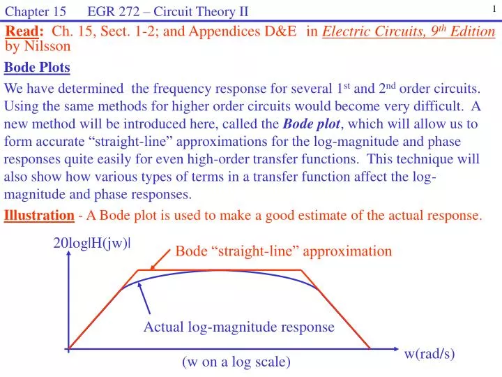
Chapter 15 EGR 272 – Circuit Theory II. 1. 20log|H(jw)|. Bode “straight-line” approximation. Actual log-magnitude response. w(rad/s). (w on a log scale). Read : Ch . 15, Sect. 1-2; and Appendices D&E in Electric Circuits, 9 th Edition by Nilsson. Bode Plots

E N D
Chapter 15 EGR 272 – Circuit Theory II 1 20log|H(jw)| Bode “straight-line” approximation Actual log-magnitude response w(rad/s) (w on a log scale) Read: Ch. 15, Sect. 1-2; and Appendices D&E in Electric Circuits, 9thEdition by Nilsson Bode Plots We have determined the frequency response for several 1stand 2nd order circuits. Using the same methods for higher order circuits would become very difficult. A new method will be introduced here, called the Bode plot, which will allow us to form accurate “straight-line” approximations for the log-magnitude and phase responses quite easily for even high-order transfer functions. This technique will also show how various types of terms in a transfer function affect the log-magnitude and phase responses. Illustration - A Bode plot is used to make a good estimate of the actual response.
Chapter 15 EGR 272 – Circuit Theory II 2 Decibels However, when scaled logs of the quantities are taken, the unit of decibels (dB), is assigned. • There are two types of Bode plots: • The Bode straight-line approximation to the log-magnitude (LM) plot, LM versus w (with w on a log scale) • The Bode straight-line approximation to the phase plot, (w) versus w (with w on a log scale)
Chapter 15 EGR 272 – Circuit Theory II 3 Standard form for H(jw): Before drawing a Bode plot, it is necessary to find H(jw) and put it in “standard form.” Show the “standard form” for H(jw) below:
Chapter 15 EGR 272 – Circuit Theory II 4 Example: Find H(jw) for H(s) shown below and put H(jw) in “standard form.”
Chapter 15 EGR 272 – Circuit Theory II 5 The additive effect of terms in H(jw): The reason that Bode plot approximations are used with the log-magnitude is due to the fact that this makes individual terms in the LM additive. The phase is also additive. Show how the LM and phase of each term in 20log|H(jw)| is additive (or acts separately). Drawing Bode plots: To draw a Bode plot for any H(s), we need to: 1) Recognize the different types of terms that can occur in H(s) (or H(jw)) 2) Learn how to draw the log-magnitude and phase plots for each type of term.
Chapter 15 EGR 272 – Circuit Theory II 6 5 types of terms in H(jw) 1) K (a constant) 2) (a zero) or (a pole) 3) jw (a zero) or 1/jw (a pole) 4) 5) Any of the terms raised to a positive integer power. Each term is now examined in detail.
Chapter 15 EGR 272 – Circuit Theory II 7 1. Constant term in H(jw) If H(jw) = K = K/0 Then LM = 20log(K) and (w) = 0 , so the LM and phase responses are: • Summary: A constant in H(jw): • Adds a constant value to the LM graph (shifts the entire graph up or down) • Has no effect on the phase
Chapter 15 EGR 272 – Circuit Theory II 8 2. A) 1 + jw/w1 (a zero): The straight-line approximations are: To determine the LM and phase responses, consider 3 ranges for w: 1) w << w1 2) w >> w1 3) w = w1
Chapter 15 EGR 272 – Circuit Theory II 9 The Bode approximations (LM and phase) for 1 + jw/w1 are shown below. Discuss the amount of error between the actual responses and the Bode approximations. • Summary: A 1 + jw/w1 (zero) term in H(jw): • Causes an upward break at w = w1 in the LM plot. There is a 0dB effect before the break and a slope of +20dB/dec or +6dB/oct after the break. • Adds 90 to the phase plot over a 2 decade range beginning a decade before w1 and ending a decade after w1. The slope is +45 deg/dec or +13.5 deg/oct.
Chapter 15 EGR 272 – Circuit Theory II 10 2B) (a pole): The straight-line approximations are: To determine the LM and phase responses, consider 3 ranges for w: 1) w << w1 2) w >> w1 3) w = w1
Chapter 15 EGR 272 – Circuit Theory II 11 The Bode approximations (LM and phase) for are shown below. Discuss the amount of error between the actual responses and the Bode approximations. • Summary: A 1 + jw/w1 (zero) term in H(jw): • Causes an downward break at w = w1 in the LM plot. There is a 0dB effect before the break and a slope of -20dB/dec or -6dB/oct after the break. • Adds -90 to the phase plot over a 2 decade range beginning a decade before w1 and ending a decade after w1. The slope is -45 deg/dec or -13.5 deg/oct.
Chapter 15 EGR 272 – Circuit Theory II 12 Example: Sketch the LM and phase plots for the following transfer function.
Chapter 15 EGR 272 – Circuit Theory II 13 Example: Sketch the LM and phase plots for the following transfer function.
Chapter 15 EGR 272 – Circuit Theory II 14 • LM: Working with slopes on Bode plots: • If the LM has a slope of 20 dB/dec, the change in LM between two frequencies can be calculated using: LM 40 dB Example:Determine the value of LM2 below. -20 dB/dec LM2 w (rad/s) 725 45
Chapter 15 EGR 272 – Circuit Theory II 15 • Phase: Working with slopes on Bode plots: • If the phase has a slope of 45 deg/dec, the change in phase (in degrees) between two frequencies can be calculated using: (deg) 90 Example:Determine the value of 2 below. -45 deg/dec 2 w (rad/s) 150 5200
Chapter 15 EGR 272 – Circuit Theory II 16 Example: Sketch the LM and phase plots for the following transfer function. (Solution provided on the following slide)
Chapter 15 EGR 272 – Circuit Theory II 17 Example: Sketch the Bode LM and phase plots for:
Chapter 15 EGR 272 – Circuit Theory II 18 Example: Sketch the LM and phase plots on the 4-cycle semi-log graph paper shown below for the following transfer function. (Pass out 2 sheets of graph paper.) Log-magnitude (LM) plot:
Chapter 15 EGR 272 – Circuit Theory II 19 Example: (continued) Phase plot:
Chapter 15 EGR 272 – Circuit Theory II 20 3A) jw term in H(jw) If H(jw) = jw = w/90 Then LM = 20log(w) and (w) = 90 Calculate 20log(w) for several values of w to show that the graph is a straight line for all frequency with a slope of 20dB/dec (or 6dB/oct). The LM and phase for H(jw) = jw are shown below. • So a jw (zero) term in H(jw) adds an upward slope of +20dB/dec (or +6dB/oct) to the LM plot. • And a jw (zero) term in H(jw) adds a constant 90 to the phase plot.
Chapter 15 EGR 272 – Circuit Theory II 21 3B) 1/(jw) term in H(jw) If H(jw) = 1/(jw) = (1/w)/-90 Then LM = 20log(1/w) = -20log(w) and (w) = -90 A few calculations could easily show that the graph of 20log(1/w)is a straight line for all frequency with a slope of -20dB/dec (or -6dB/oct). The LM and phase for H(jw) = 1/(jw) are shown below. • So a 1/(jw) (pole) term in H(jw) adds a downward slope of -20dB/dec (or -6dB/oct) to the LM plot. • And a 1/(jw) (pole) term in H(jw) adds a constant -90 to the phase plot.
Chapter 15 EGR 272 – Circuit Theory II 22 Example: Sketch the LM and phase plots for the following transfer function.
Chapter 15 EGR 272 – Circuit Theory II 23 Example: Sketch the LM and phase plots for the following transfer function.
Chapter 15 EGR 272 – Circuit Theory II 24 Calculation of exact points to check Bode Plots Evaluating H(jw) at a particular value of w is helpful to check Bode Plots. An example is shown below.
Chapter 15 EGR 272 – Circuit Theory II 25 Example: Evaluate the H(jw) on the last page at w = 500 rad/s and w = 8000 rad/s. Compare the values with the Bode plots. Do they appear to be correct?
Chapter 15 EGR 272 – Circuit Theory II 26 5. Poles and zeros raised to an integer power in H(s) In the last class it was demonstrated that terms in H(jw) are additive. Therefore, a double terms (such as a pole or zero that is squared) simply acts like two terms, a triple term acts like three terms, etc. Illustration: Show that (1 + jw/w1)N results in the following responses: LM plot: Has a 0dB contribution before its break frequency Will increase at a rate of 20NdB/dec after the break There will be an error of 3NdB at the break between the Bode straight-line approximation and the exact LM Phase plot: Has a 0 degree contribution until 1 decade before its break frequency Will increase at a rate of 45Ndeg/dec for two decades (from 0.1w1 to 10w1). The total final phase contribution will be 90N degrees.
Chapter 15 EGR 272 – Circuit Theory II 27 So (1 + jw/w1)N results in the following responses:
Chapter 15 EGR 272 – Circuit Theory II 28 Example: Sketch the LM plot for the following transfer function.
Chapter 15 EGR 272 – Circuit Theory II 29 Generating LM and phase plots using Excel and MATLAB: Refer to the handout entitled “Frequency Response” which includes detailed examples of creating LM and phase plots using Excel and MATLAB. Generating LM and phase plots using PSPICE: Refer to the handout entitled “PSPICE Example: Frequency Response (Log-Magnitude and Phase)” which includes a detailed example of creating LM and phase plots using PSPICE.
Chapter 15 EGR 272 – Circuit Theory II 30 Bode Plots - Recall that there are 5 types of terms in H(s). The first four have already been covered. 5.Complex terms in H(s) A second order term in H(s) with complex roots has the general form s2 + 2s + wo2 . After factoring out the constant has the wo2 , the corresponding term in H(jw) is: Key point: The complex term above is identical to a double real pole or a double real zero in the Bode straight-line approximation, but they differ in the exact curves.
Chapter 15 EGR 272 – Circuit Theory II 31 Complex peaks and damping ratio Exercise: Complete the table below showing the value of the complex peak (for a complex zero) * z = 1 is not complex. It corresponds to a double-zero.
Chapter 15 EGR 272 – Circuit Theory II 32 The following graphs from the text (Electric Circuits, 9thEdition, by Nilsson) below show the Bode straight-line approximation and the exact curve for different values of z.
Chapter 15 EGR 272 – Circuit Theory II 33 Example: Sketch the LM responses for H1(s), which has a double zero, and H2(s), which has a complex zero. A) Find H1(jw) and sketch the LM response
Chapter 15 EGR 272 – Circuit Theory II 34 Example: Sketch the LM responses for H1(s), which has a double zero, and H2(s), which has a complex zero. B) Find H2(jw) and sketch the LM response
Chapter 15 EGR 272 – Circuit Theory II 35 Filter order Unfortunately, we can’t build ideal filters. However, the higher the order of a filter, the more closely it will approximate an ideal filter. The order of a filter is equal to the degree of the denominator of H(s). (Of course, H(s) must also have the correct form.) LM Ideal LPF slope = 4th-order LPF slope = -80dB/dec 3rd-order LPF slope = -60dB/dec 2nd-order LPF slope = -40dB/dec 1st-order LPF slope = -20dB/dec w wC
Chapter 15 EGR 272 – Circuit Theory II 36 Recognizing filter types from the transfer function Low-pass filter (LPF) - Discuss the form of LM, H(jw), and H(s). High-pass filter (HPF) - Discuss the form of LM, H(jw), and H(s).
Chapter 15 EGR 272 – Circuit Theory II 37 Band-pass filter (BPF) - Discuss the form of LM, H(jw), and H(s). Band-stop filter (BSF) - Discuss the form of LM, H(jw), and H(s). Also define a “notch” filter.
Chapter 15 EGR 272 – Circuit Theory II 38 Practical Filter Examples: Discuss a stereo tuner, 5-band equalizer, 60 Hz interference block.
Chapter 15 EGR 272 – Circuit Theory II 39 Active and passive filters Passive filter - a filter constructed using passive circuit elements (R’s, L’s, and C’s) Active filter - a filter constructed using active circuit elements (primarily op amps) Analysis of active filters Active filters are fairly easy to analyze. Recall that a resistive inverting amplifier circuit has the following relationship: Replacing the resistors with impedances yields a transfer function, H(s):
Chapter 15 EGR 272 – Circuit Theory II 40 Example: Find H(s) =Vo(s)/Vin(s) for the circuit below and sketch the LM response.
Chapter 15 EGR 272 – Circuit Theory II 41 Impedance and Frequency Scaling Filter tables are commonly available that list component values for various types of filters. However, the tables could not possibly list component values for all possible cutoff frequencies. Typically, filter tables will list cutoff frequencies of perhaps 1 Hz or 1 kHz. The user can then scale the cutoff frequencies to the desired values using frequency scaling. Similarly, component values may be too large or too small (for example, a filter might be shown using 1 ohm resistors or 1F capacitors) so the components need to be scaled using impedance scaling.
Chapter 15 EGR 272 – Circuit Theory II 42 sL R Z(s) Impedance Scaling – a procedure used to change the impedance of a circuit without affecting its frequency response. Consider the series RLC circuit shown below. Show that to scale the impedance by a factor KZ :
Chapter 15 EGR 272 – Circuit Theory II 43 + sL + Vi(s) R Vo(s) _ _ Frequency Scaling – a procedure used to scale all break frequencies in the frequency response of a circuit. The frequency response is scaled without affecting the circuit impedance (the impedance is the same at the original and new break frequencies). Consider the series RLC circuit shown below. As seen in an earlier class, H(s) is described below. Note that H(s) described above is the transfer function of a band-pass filter. The LM is shown on the following page.
Chapter 15 EGR 272 – Circuit Theory II 44 LM of the original band-pass filter (center frequency = wo): LM of the frequency-scaled band-pass filter (center frequency = KFwo):
Chapter 15 EGR 272 – Circuit Theory II 45 Show that to scale the frequency by a factor KF :
Chapter 15 EGR 272 – Circuit Theory II 46 Example: Impedance and frequency scaling. A) Determine H(s) = Vo(s)/Vi(s) B) Sketch the LM response
Chapter 15 EGR 272 – Circuit Theory II 47 Example: (continued) C) A cutoff frequency of 1 rad/s and component values of 1 ohm and 1 Farad are not very useful. Scale the frequency so that the cutoff frequency is 500 rad/s. Also use a 1 k resistor instead of a 1 resistor.
Chapter 15 EGR 272 – Circuit Theory II 48 Example: (continued) D) Draw the new circuit. Determine the new H(s) and verify that the LM response has been shifted as planned. E) Calculate the circuit impedance at the break frequency for the new circuit and compare it to the circuit impedance at the break frequency for the original circuit.