Download
1 / 82
870 likes | 1.23k Views
Decibels, Filters, and Bode Plots. OBJECTIVES. Develop confidence in the use of logarithms and decibels in the description of power and voltage levels.

E N D
OBJECTIVES • Develop confidence in the use of logarithms and decibels in the description of power and voltage levels. • Become familiar with the frequency response of high- and low-pass filters. Learn to calculate the cutoff frequency and describe the phase response. • Be able to calculate the cutoff frequencies and sketch the frequency response of a pass-band, stop-band, or double-tuned filter. • Develop skills in interpreting and establishing the Bode response of any filter. • Become aware of the characteristics and operation of a crossover network.
INTRODUCTION • The unit decibel (dB), defined by a logarithmic expression, is used throughout the industry to define levels of audio, voltage gain, energy, field strength, and so on.
INTRODUCTIONLogarithms • Basic Relationships • Let us first examine the relationship between the variables of the logarithmic function. • The mathematical expression:
INTRODUCTIONLogarithms • Some Areas of Application • The following are some of the most common applications of the logarithmic function: • 1. The response of a system can be plotted for a range of values that may otherwise be impossible or unwieldy with a linear scale. • 2. Levels of power, voltage, and the like can be compared without dealing with very large or very small numbers that often cloud the true impact of the difference in magnitudes. • 3. A number of systems respond to outside stimuli in a nonlinear logarithmic manner. • 4. The response of a cascaded or compound system can be rapidly determined using logarithms if the gain of each stage is known on a logarithmic basis.
FIG. 21.1 Semilog graph paper. INTRODUCTIONLogarithms
FIG. 21.2 Frequency log scale. INTRODUCTIONLogarithms
FIG. 21.4 Example 21.1. FIG. 21.3 Finding a value on a log plot. INTRODUCTIONLogarithms
PROPERTIES OF LOGARITHMS • There are a few characteristics of logarithms that should be emphasized: • The common or natural logarithm of the number 1 is 0 • The log of any number less than 1 is a negative number • The log of the product of two numbers is the sum of the logs of the numbers • The log of the quotient of two numbers is the log of the numerator minus the log of the denominator • The log of a number taken to a power is equal to the product of the power and the log of the number
PROPERTIES OF LOGARITHMSCalculator Functions • Using the TI-89 calculator, the common logarithm of a number is determined by first selecting the CATALOG key and then scrolling to find the common logarithm function. • The time involved in scrolling through the options can be reduced by first selecting the key with the first letter of the desired function—in this case, L, as shown below, to find the common logarithm of the number 80.
DECIBELS • Power Gain • Voltage Gain • Human Auditory Response
TABLE 21.1 DECIBELS
TABLE 21.2 Typical sound levels and their decibel levels. DECIBELS
FIG. 21.5 LRAD (Long Range Acoustic Device) 1000X. (Courtesy of the American Technology Corporation.) DECIBELS
FIG. 21.6 Defining the relationship between a dB scale referenced to 1 mW, 600Ωand a 3 V rms voltage scale. DECIBELSInstrumentation
FILTERS • Any combination of passive (R, L, and C) and/or active (transistors or operational amplifiers) elements designed to select or reject a band of frequencies is called a filter. • In communication systems, filters are used to pass those frequencies containing the desired information and to reject the remaining frequencies.
FILTERS • In general, there are two classifications of filters: • Passive filters • Active filters
FIG. 21.7 Defining the four broad categories of filters. FILTERS
FIG. 21.9 R-C low-pass filter at low frequencies. FIG. 21.8 Low-pass filter. R-C LOW-PASS FILTER
FIG. 21.10 R-C low-pass filter at high frequencies. FIG. 21.11 Vo versus frequency for a low-pass R-C filter. R-C LOW-PASS FILTER
FIG. 21.12 Normalized plot of Fig. 21.11. R-C LOW-PASS FILTER
FIG. 21.13 Angle by which Vo leads Vi. R-C LOW-PASS FILTER
FIG. 21.14 Angle by which Vo lags Vi. R-C LOW-PASS FILTER
FIG. 21.15 Low-pass R-L filter. FIG. 21.16 Example 21.5. R-C LOW-PASS FILTER
FIG. 21.17 Frequency response for the low-pass R-C network in Fig. 21.16. R-C LOW-PASS FILTER
FIG. 21.18 Normalized plot of Fig. 21.17. R-C LOW-PASS FILTER
FIG. 21.19 High-pass filter. R-C HIGH-PASS FILTER
FIG. 21.20 R-C high-pass filter at very high frequencies. FIG. 21.21 R-C high-pass filter at f =0 Hz. R-C HIGH-PASS FILTER
FIG. 21.22 Vo versus frequency for a high-pass R-C filter. R-C HIGH-PASS FILTER
FIG. 21.23 Normalized plot of Fig. 21.22. R-C HIGH-PASS FILTER
FIG. 21.24 Phase-angle response for the high-pass R-C filter. R-C HIGH-PASS FILTER
FIG. 21.25 High-pass R-L filter. R-C HIGH-PASS FILTER
FIG. 21.26 Normalized plots for a low-pass and a high-pass filter using the same elements. R-C HIGH-PASS FILTER
FIG. 21.27 Phase plots for a low-pass and a high-pass filter using the same elements. R-C HIGH-PASS FILTER
FIG. 21.28 Series resonant pass-band filter. PASS-BAND FILTERS
FIG. 21.29 Parallel resonant pass-band filter. PASS-BAND FILTERS
FIG. 21.30 Series resonant pass-band filter for Example 21.7. PASS-BAND FILTERS
FIG. 21.31 Pass-band response for the network. PASS-BAND FILTERS
FIG. 21.32 Normalized plots for the pass-band filter in Fig. 21.30. PASS-BAND FILTERS
FIG. 21.33 Pass-band filter. PASS-BAND FILTERS
FIG. 21.34 Pass-band characteristics. PASS-BAND FILTERS
FIG. 21.36 Pass-band characteristics for the filter in Fig. 21.35. FIG. 21.35 Pass-band filter. PASS-BAND FILTERS
FIG. 21.37 Network of Fig. 21.35 at f =994.72 kHz. PASS-BAND FILTERS
BAND-REJECT FILTERS • Since the characteristics of a band-reject filter (also called stop-band or notch filter) are the inverse of the pattern obtained for the band-pass filter, a band-reject filter can be designed by simply applying Kirchhoff’s voltage law to each circuit.
FIG. 21.38 Demonstrating how an applied signal of fixed magnitude can be broken down into a pass-band and band-reject response curve. BAND-REJECT FILTERS
FIG. 21.39 Band-reject filter using a series resonant circuit. BAND-REJECT FILTERS
FIG. 21.40 Band-reject filter using a parallel resonant network. BAND-REJECT FILTERS
FIG. 21.41 Band-reject filter. BAND-REJECT FILTERS
FIG. 21.42 Band-reject characteristics. BAND-REJECT FILTERS
DOUBLE-TUNED FILTER • Some network configurations display both a pass-band and a stop-band characteristic, such as shown in Fig. 21.43. • Such networks are called double-tuned filters.