Download
1 / 20
200 likes | 317 Views
This study presents the results obtained from conducting a magnetic analysis of a multilayered sample structure composed of various metals (Ta, Cu, Co, Ni, Pt). The measurements were performed at a low temperature of 4 degrees, assessing R versus t measurements under different magnetic field strengths. A simple three-dipole model was employed to understand the transitions between two stable magnetic states characterized by uniaxial anisotropies. The analysis highlights the significance of dipole placement and interaction in shaping the film's magnetic behavior, paving the way for future advancements in magnetic materials.

E N D
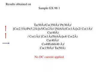
Results obtained on Sample GX 98 1 Ta(50Å)/Cu(350Å)/ Pt(30Å)/ [Co(2.5Å)/Pt(5.2Å)]x5/Co(2Å)/ [Ni(6Å)/Co(1Å)]x2/ Co(1Å)/ Cu(40Å) / Co(1Å)/ [Co(1Å)/Ni(6Å)]x4/ Co(2Å) Cu(40Å)/ Co40Fe60(40 Å)/ Cu(150Å)/ Ta(50Å) No DC current applied
At 4 degres of the axe that was suppose to be the direction perpendicular to the film plane
5 degres 6 degres
From the following model it looks that we are observing transition between the two following states
Simple three-dipole model Three magnetic dipoles µi (i = 1,2,3) located on the vertical axis z, with first order uniaxial anisotropies of magnitudes ki and axis z. Distances between dipoles are dij (i j) For each dipole, the energy writes: Total Energy: Dipole 1 : k1 = 6×10⁶ erg/cm2 (=K×t), µ1 = 1800 emu/cm2 (=MS×t, with t in nm) Dipole 2 : k2 = 3×10⁵ erg/cm2 (=K×t), µ2 = 900 emu/cm2 (=MS×t, with t in nm) Dipole 3 : k3 = -3×10⁶ erg/cm2 (=K×t), µ3 = 1800 emu/cm2 (=MS×t, with t in nm) Distances: d12 = 3 nm, d22 = 3 nm, d13 = d12 + d23 = 6 nm
qH = 0° H -5000 Oe -2500 Oe -2600 Oe -100 Oe +100 Oe +2500 Oe +7700 Oe +7800 Oe Increasing field branch
qH = +1° H -5000 Oe -2500 Oe -100 Oe +100 Oe +3000 Oe +3100 Oe +6000 Oe +6100 Oe Increasing field branch
qH = +6° H Field ranges exist where two magnetic states are stable. They essentially differ in the orientation of the magnetization of the layer with in-plane anisotropy -1400 Oe H H +1200 Oe H H