The Thermodynamic Diagram
780 likes | 1.09k Views
The Thermodynamic Diagram. Adapted by K. Droegemeier for METR 1004 from Lectures Developed by Dr. Frank Gallagher III OU School of Meteorology. What is it?.

The Thermodynamic Diagram
E N D
Presentation Transcript
The Thermodynamic Diagram Adapted by K. Droegemeier for METR 1004 from Lectures Developed by Dr. Frank Gallagher III OU School of Meteorology
What is it? • The thermodynamic diagram, of which there exist many types, is a chart that allows meteorologists to easily assess, via quantitative graphical analysis, the stability and other properties of the atmosphere given a vertical profile of temperature and moisture (i.e., a sounding).
Stve Diagram to be used in this class
What Can it Be Used to Estimate? • Cloud base and cloud top height • Expected intensity of updrafts, downdrafts, and outflow winds • Likelihood of hail • Storm and cloud type (supercell, multicell, squall line) • Storm motion • Likelihood of turbulence • Likelihood of storm updraft rotation • 3D location of clouds • Precipitation amount • High temperature • Destabilization via advection, subsidence • And many others….
The Stuve Diagram • Construction: Altitude in Km or 1,000’s of feet Pressure levels in mb. -400 C +300 C Temperature How high is the 500 mb level?
Stve Diagram to be used in this class
Thermodynamic Diagram • Saturation mixing ratio line (yellow): p It provides the saturation mixingratio associated with the dry bulbtemperature, or the mixing ratioassociated with the dew point.The same line provides both T
Stve Diagram to be used in this class
Thermodynamic Diagram • Saturation mixing ratio line (yellow): p It provides the saturation mixingratio associated with the dry bulbtemperature, or the mixing ratioassociated with the dew point.The same line provides both T What is ws at p=1000 mb and T=-100 C? What is the RH at 1000 mb when T=240 C and Td=130 C? If T=200 C and RH = 70%, what is Td at 1000 mb?
Thermodynamic Diagram p • Dry adiabats (green): Unsaturated air that rises or sinksdoes so parallel to the dry adiabats.This line simply shows the rate oftemperature decrease with height foran unsaturated parcel. T
Stve Diagram to be used in this class
Thermodynamic Diagram p • Dry adiabats (green): Unsaturated air that rises or sinksdoes so parallel to the dry adiabats.This line simply shows the rate oftemperature decrease with height foran unsaturated parcel. T What is the temperature of an unsaturated air parcel at 1000 mb and T=200C if lifted to 900 mb? to 600 mb? What will be the temperature of an unsaturated air parcel at 600 mb and T= -200C if it sinks to 1000 mb?
Temperature of a parcel at 1000 mb Tparcel = 20C
Temperature of a parcel at 1000 mb Tparcel = 20C
Parcel is unsaturated, so if liftedto 600 mb, it follows parallel toa dry adiabat (green line) – notethat the parcel goes parallel tothe NEAREST green line. Temperature of a parcel at 1000 mb Tparcel = 20C
Temperature of a parcel lifted dry adiabatically to 600 mb. Tparcel = -20C Temperature of a parcel at 1000 mb Tparcel = 20C
Thermodynamic Diagram • Moist (pseudo) adiabats (red): Saturated air that rises or sinksdoes so parallel to the moist adiabats.This line simply shows the rate oftemperature decrease with height fora saturated parcel. p T
Stve Diagram to be used in this class
Thermodynamic Diagram • Moist (pseudo) adiabats (red): Saturated air that rises or sinksdoes so parallel to the moist adiabats.This line simply shows the rate oftemperature decrease with height fora saturated parcel. p T Problem: (a) Moist air rising from the surface (T=12oC) will have a temperature of _________ at 1 km. (b) If dry, the temperature will be? Why? (a) T = 12oC + (-6oC km-1) x (1 km) = 6oC (b) T = 12oC + (-10oC km-1) x (1 km) = 2oC
Using the Thermodynamic Diagram to Assess Atmospheric Stability
The Thermodynamic Diagram • We’ll use two types of thermodynamic diagrams in this class. • The simpler of the two is the Stve diagram, and we’ll use this to familiarize you with the use of such diagrams • The more popular (in the U.S.) and more useful is the Skew-T Log-p diagram, which we’ll apply later.
Stve diagram Green Dry Adiabats Red Moist Adiabats Yellow Saturation Mixing Ratio
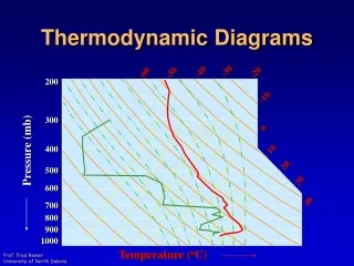
Thermodynamic Diagram • Stability: To determine the stability you must plot a sounding. A sounding is the temperature at various heights as measured by a balloon-borne radiosonde. p The sounding is also called the environmental lapse rate (ELR). COLD WARM T Note: We also plot dew point on the chart -- we’ll get to that later.
Types of Stability Unsat Sat
Example: Dry Neutral Neutral to Dry Processes Unstable to Moist Processes ELR
Example: Moist Neutral Stable to Dry Processes Neutral to Moist Processes ELR
Example: Absolutely Unstable Unstable to Dry Processes Unstable to Moist Processes ELR
Example: Conditionally Unstable Stable to Dry Processes Unstable to Moist Processes ELR
Example: Absolutely Stable Stable to Dry Processes Stable to Moist Processes ELR
Norman Sounding3 February 1999 Temperature Sounding Dew Point Sounding
Definitions • Lifting Condensation Level (LCL) • The level to which a parcel must be raised dry adiabatically, and at constant mixing ratio, in order to achieve saturation • It is determined by lifting the surface dew point upward along a mixing ratio line, and the surface temperature upward along a dry adiabat, until they intersect.
Example: LCL Notes: Dry adiabatic ascent from surface Constant mixing ratioRH increasesas parcelascends (T and Td approachone another; RH is 100% at LCL Surface Data T= 10oC Td = 3oC Mixing Ratio = 5 g kg-1 Data at LCL TLCL = 2oC Mixing Ratio = 5 g kg-1 LCL = 900 mb Td T
Definitions • Lifting Condensation Level (LCL) • The LCL is CLOUD BASE HEIGHT for a parcel lifted mechanically, e.g., by a front. Remember, it is the LIFTED OR LIFTING condensation level.
Example: LCL Notes: Dry adiabatic ascent from surface Constant mixing ratioRH increasesas parcelascends (T and Td approachone another; RH is 100% at LCL Surface Data T= 10oC Td = 3oC Mixing Ratio = 5 g kg-1 LCL = 900 mb Td T
Definitions • Level of Free Convection (LFC) • The level to which a parcel must be lifted in order for its temperature to become equal to that of the environment. • It is found by lifting a parcel vertically until it becomes saturated, and then lifting it further until the temperature of the parcel crosses the ELR
Example: LFC LFC = 840 mb LCL = 900 mb Surface Data T= 10oC Td = 3oC Mixing Ratio = 5 g kg-1 Td T
Definitions • Level of Free Convection (LFC) • Any subsequent lifting will result in the parcel being warmer than the environment, i.e., instability. • This is what “free convection” means – the parcel will convect freely after reaching the LFC
Example: LFC LFC = 840 mb LCL = 900 mb Surface Data T= 10oC Td = 3oC Mixing Ratio = 5 g kg-1 Td T
Definitions • Equilibrium Level • A level higher than the LFC above which the temperature of a rising parcel becomes equal to that of the environment, i.,e. the parcel has zero buoyancy or is in equilibrium with the environment • It is found by lifting a parcel until its temperature becomes equal to the ELR
Example: LFC and EL EL = 580 mb LFC = 840 mb LCL = 900 mb Surface Data T= 10oC Td = 3oC Mixing Ratio = 5 g kg-1 Td T
Definitions • Equilibrium Level • Any subsequent lifting above the EL leads to stability • The EL marks the “top” of thunderstorms, though in reality the upward momentum of updraft air makes thunderstorms overshoot the EL (overshooting top)
Example: LFC and EL EL = 580 mb LFC = 840 mb LCL = 900 mb Surface Data T= 10oC Td = 3oC Mixing Ratio = 5 g kg-1 Td T
Definitions • Convective Condensation Level • The level at which convective clouds will form due to surface heating alone. • It is found by taking the surface dew point upward along a mixing ratio line until it intersects the ELR. • Convective Temperature (Tc) • The temperature required at the ground for convective clouds to form. • It is found by taking a parcel at the CCL downward along a dry adiabat to the surface.
Example: LCL, CCL, and Tc CCL = 750 mb LCL = 900 mb Surface Data T= 10oC Td = 3oC Mixing Ratio = 5 g kg-1 Tc = 23oC Td T
Example: Positive and Negative Areas EL = 510 mb Parcel warmer than environment! Positive Area Negative Area Need to push parcel up!!!! LFC = 800 mb Surface Data T= 10oC Td = 3oC Mixing Ratio = 5 g kg-1 LCL = 900 mb Td T