Download
1 / 56
560 likes | 598 Views
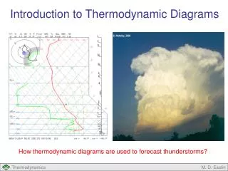
Explore the key characteristics, advantages, and transformations involved in using thermodynamic diagrams to depict atmospheric processes. Learn about different types of diagrams and their applications.

E N D
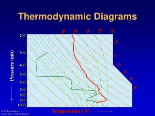
-30 -40 -20 -50 -60 200 -10 300 0 Pressure (mb) 400 10 20 500 30 600 40 700 800 900 1000 Temperature (oC) Thermodynamic Diagrams
Thermodynamic Diagrams • Reading • Hess • Chapter 5 • pp 65 – 74 • Tsonis • pp 143 – 150 • Air Weather Service,AWS/TR-79/006 • Wallace & Hobbs • pp 78 – 79
Thermodynamic Diagrams • Objectives • Be able to list the three desirable characteristics of a thermodynamic diagram • Be able to describe how a transformation is made from p, a coordinates when designing a thermodynamic diagram
Thermodynamic Diagrams • Objectives • Be able to list the coordinates of each thermodynamic diagram • Be able to describe the advantages and disadvantages of each thermodynamic diagram
Thermodynamic Diagrams • Provide a graphical representation of thermodynamic processes in the atmosphere
Thermodynamic Diagrams • Thermodynamic Processes? • Isobaric • Isothermal • Dry Adiabatic • Pseudoadiabatic • Constant Mass
Thermodynamic Diagrams • Thermodynamic Diagrams • Eliminates or simplifies calculations
Pressure (mb) Temperature (oC) Thermodynamic Diagrams • Most Simplistic 400 500 600 Temp. 700 800 Dew Point 900 1000 -20 -10 0 10 20 30
Pressure (mb) Temperature (oC) Thermodynamic Diagrams • Not very useful 400 500 600 Temp. 700 800 Dew Point 900 1000 -20 -10 0 10 20 30
Thermodynamic Diagrams • Desirable Characteristics • Area Equivalent • Area enclosed by a cyclic process is proportional to energy
-30 -40 -20 -50 -60 200 -10 300 0 Pressure (mb) 400 10 20 500 30 600 40 700 800 900 1000 Temperature (oC) Desirable Characteristics
Desirable Characteristics • As many isopleths as possible be straight lines
Temperature (oC) Desirable Characteristics -30 -40 -20 -50 -60 200 -10 300 0 Pressure (mb) 400 10 20 500 30 600 40 700 800 900 1000
Desirable Characteristics • The angle between isotherms and adiabats be as large as possible • Sensitivity to the rate of change of temperature with pressure in the vertical • Easier to determine stability of the environment • 90o Optimum
Temperature (oC) Desirable Characteristics -30 -40 -20 -50 -60 -10 0 Pressure (mb) 10 20 30 40
Coordinates • Select so that it satisfies Area Equivalent characteristic • Enclosed area is proportional to energy • Use p & a
Coordinates • Known as Clapeyron Diagram • Small angle between T & q q1 T1 q2 T2 P Dry Adiabats 1000 mb a
P A a B Coordinates • Equal Area Transformation • Consider two other variables A & B
P A a B Coordinates • Equal Area Transformation • Create a transformation from -p, a to A, B
P a Equal Area Transformation A B
Equal Area Transformation • Closed integral cannot equal zero unless it is an exact differential
Equal Area Transformation • Differentiate s with respect to a and B • So ...
Equal Area Transformation • Differentiate p with respect to B • Differentiate A with respect to a
Equal Area Transformation • Specify B, can determine A • Equal Area maintained
Emagram • Energy per Unit Mass Diagram • Set B = T
Emagram • Using the Ideal Gas Law • Differentiate
Emagram • Integrate
Emagram • Once again, the Equation of State • Take the natural logarithm
Emagram • Substitute
Emagram • Select f(t) such that • Finally … coordinates A & B are …
Emagram 400 mb 100oC 80oC qe 60oC 600 mb 40oC Pressure 20oC w q = 0oC 800 mb -20oC 1000 mb -40oC -20oC 0oC 20oC 40oC Temperature
Emagram • Area proportional to energy • Four sets of straight (or nearly straight) lines • 45o angle between adiabats and isotherms
Tephigram • T- f Diagram • Temperature = T • Entropy = f
Tephigram • Coordinates • Similar to Emagram • Different constant of integration
Tephigram • Evaluate f(T) using Potential Temperature • Ideal Gas Law • Substitute for p
Tephigram • Take the natural logarithm
Tephigram • Solve for lna
Tephigram • Solve for lna
Tephigram • Select f(T) • Substitute
Tephigram • Substitute • Since g(T) = -f(T)
Tephigram • Coordinates • Similar to Emagram
Tephigram Temperature -20oC -40oC 400 mb 60oC 0oC qe 40oC 600 mb Pressure 20oC 800 mb w q = 0oC 1000 mb
Tephigram • Area proportional to energy • Four sets of straight (or nearly straight) lines • Isobars Curved! • 90o angle between adiabats and isotherms
Skew-T Log-P • Modified Emagram • Isotherm-Adiabat angle 90o • Set B = -R lnp
Skew-T Log-P • But... • So ... • Becomes ..
Skew-T Log-P • Multiply both sides by da
Skew-T Log-P • Integrate • Ideal Gas Law
Skew-T Log-P • Select f(lnp) K = arbitrary constant
Skew-T Log-P • Coordinates • Similar to Emagram