Download
1 / 59
670 likes | 1.46k Views
Regression Analysis Fitting Models to Data. CHEE 209 Module 5. Outline . types of models least squares estimation - assumptions fitting a straight line to data least squares parameter estimates graphical diagnostics quantitative diagnostics multiple linear regression

E N D
Regression AnalysisFitting Models to Data CHEE 209 Module 5 K. McAuley
Outline • types of models • least squares estimation - assumptions • fitting a straight line to data • least squares parameter estimates • graphical diagnostics • quantitative diagnostics • multiple linear regression • least squares parameter estimates • diagnostics • precision of parameter estimates and predicted responses K. McAuley
Empirical Modeling - Terminology • response • dependent variable that responds to changes in other variables • the response is the model output that we are trying to predict • explanatory variable • independent variable, regressor variable, input, factor • these are the quantities that we believe have an influence on the response • parameter • coefficients in the model that describe how the independent variables influence the response K. McAuley
Models When we are estimating a model from data, we consider the following form: response random error parameters explanatory variables K. McAuley
The Random Error Term • is included to reflect the fact that measured data contain variability • successive experiments conducted under the same conditions (values of the explanatory variables) are likely to give slightly different results • this is the random component • random error is not necessarily the result of mistakes in experimental procedures. It’s just a reflection of inherent variability K. McAuley
Types of Models • linear/nonlinear in the parameters • linear/nonlinear in the explanatory variables • number of response variables • single response (standard regression) • multi-response (or “multivariate” models) From the perspective of statistical model-building, the key point is whether the model is linear or nonlinear in the PARAMETERS. K. McAuley
Linear Regression Models A model that is linear in the parameters can be nonlinear in the regressors K. McAuley
Nonlinear Regression Models • nonlinear in the parameters • e.g., Arrhenius rate expression nonlinear linear (if E is fixed) K. McAuley
Ordinary LS vs. Multi-Response • single response (ordinary least squares) • multi-response We will be focussing on single response models. K. McAuley
Fitting a Straight Line to Data Consider some data Goal - predict solder thickness as a function of temperature The trend appears to be quite linear --> try fitting a straight- line model to these data Y - thickness x - temperature K. McAuley
Estimating a Model • How to measure the effectiveness of model predictions? • prediction error = measured response - predicted value • Sometimes the prediction error is positive and sometimes negative. • Squared prediction error is always positive • Small squared prediction errors are better than large ones • Least-squares estimation involves selecting model parameters to make the sum of the squared prediction errors as small as possible K. McAuley
Least Squares Estimation - graphically least squares - minimize sum of squared prediction errors o Model predictions response (solder thickness) o o o o o T prediction error “residual” K. McAuley
Assumptions for Least Squares Estimation 1. Values of explanatory variables are known EXACTLY • e.g. If we are studying the effect of temperature on yield, we assume that we can achieve the desired reactor temperature without any error. • random error is strictly in the response variable • practically - a random component will almost always be present in the explanatory variables as well • we assume that this random component in the experimental settings has a substantially smaller effect on the response than the random component in the response • if random fluctuations in the independent variables are important, we should use more complicated techniques (e.g. “Errors-in-Variables” approach) K. McAuley
Assumptions for Least Squares Estimation 2. The form of the equation provides an adequate representation for the data • We assume that this is true and fit the model • Look for evidence that the model is inadequate after estimating the parameters to check the validity of the assumption 3. Variance of random error is CONSTANT over range of data collected • e.g., variance of random fluctuations in thickness measurements at high temperatures is the same as variance at low temperatures • if the variance is not constant, a more complex estimation procedure is required • We assume that the assumption is valid and use the prediction errors to test the validity of the assumption K. McAuley
Assumptions for Least Squares Estimation 4. The random fluctuations in each measurement are statistically independent from those of other measurements • e.g. if we do a set of experiments at different temperatures and measure the resulting yields, the random error in the yield for experiment 3 doesn’t depend on what happened in experiment 2. K. McAuley
Assumptions for Least Squares Estimation 5. Random error term, , is normally distributed • not essential for least-squares estimation • important when determining confidence intervals for parameter estimates and model predictions Random error is “independent, identically distributed” (I.I.D) -- statisticians say that the random error is IID Normal K. McAuley
More Notation and Terminology Capitals - Y - denotes a random variable Lower case - y, x - denotes measured values of variables Model Measurement K. McAuley
More Notation and Terminology Estimate - denoted by “hat” • examples - estimates of response, parameter Residual - difference between measured and predicted response K. McAuley
Least Squares Estimation (for one explanatory variable) Find the parameter values that minimize the sum of squares of the residuals over the data set, e.g:Solution • Take derivatives of SSE with respect to the model parameters 0 and 1 • When SSE is minimized, the derivatives with respect to the parameters are zero • Solve two equations in two unknowns for 0 and 1 • M&R&H 3rd ed. 267-268 M&R 3rd ed. 376-377 K. McAuley
Least-Squares Parameter Estimates (for case of one explanatory variable) Note that the parameter estimates are functions of BOTH the explanatory variable values and the measured response values. The estimates are random variables because they depend on noisy data. K. McAuley
Multiple Linear Regression • Least-Squares Estimation for models with more than one regressor variable, e.g. or Use a matrix approach for linear regression when there is more than one input variable in the model. K. McAuley
Multiple Linear Regression Suppose there are k regressor variables and n observations: This system of n equations can be written in matrix notation as: K. McAuley
Multiple Linear Regression In matrix form: K. McAuley
Multiple Linear Regression If we have estimates of the parameters, we can calculate the model predictions from: Minimizing the sum of squared residuals requires solving (p. 417 in M&R, but not in matrix form in M&R&H): to get K. McAuley
Multiple Linear Regression How do we get the solution below? Use the data set to determine the X and y matrices and solve for the parameter estimates. This is how Excel, JMP and other statistical packages estimate parameters. K. McAuley
Diagnostics - Graphical Basic Principle – a good model should extract as much trend as possible from the data Residuals should have no remaining trend - • with respect to the explanatory variables • with respect to the data sequence number • with respect to other possible explanatory variables (“secondary variables”) • with respect to predicted values K. McAuley
Graphical Diagnostics Residuals vs. Predicted Response Values - even scatter over range of prediction - no discernable pattern - roughly half the residuals are positive, half negative * * residual ei * * * * * * * * * * * * DESIRED RESIDUAL PROFILE K. McAuley
Graphical Diagnostics Residuals vs. Predicted Response Values * outlier lies outside main body of residuals residual ei * * * * * * * * * * * * * RESIDUAL PROFILE WITH OUTLIERS K. McAuley
Graphical Diagnostics Residuals vs. Predicted Response Values variance of the residuals appears to increase with higher predictions * * * residual ei * * * * * * * * * * * * * * * * * * NON-CONSTANT VARIANCE K. McAuley
Graphical Diagnostics Residuals vs. Explanatory Variables • ideal - no systematic trend present in plot • inadequate model - evidence of trend present left over trend - need quadratic term in model? * residual ei * * * * * * * * x * * * K. McAuley
Graphical Diagnostics Residuals vs. Explanatory Variables Not in Model • ideal - no systematic trend present in plot • inadequate model - evidence of trend present * residual ei * * * * * * w * * * * * * * systematic trend not accounted for in model - include a linear term in “w” K. McAuley
Graphical Diagnostics Residuals vs. Order of Data Collection * failure to account for time trend in data residual ei * * * * * * * t * * * * * K. McAuley
Quantitative Lack of Fit and Model Adequacy Tests • Are the residuals large enough to indicate that the model is imperfect? • Compare residuals and s2 from replicates * * * * * * * * * * K. McAuley
Quantitative Lack of Fit and Model Adequacy Tests • Is the model really better than no model at all? • Compare variability explained by model with variability remaining in residuals * * * * * * * * * * K. McAuley
Quantitative Diagnostics - Ratio Tests (not in text) Is the variance of the residuals large enough to indicate that the model is imperfect? • If the model is perfect, the variance of the residuals should be the same as the variance of measured responses when repeated experiments are performed at a constant set of operating conditions. • Compare variance of residuals relative to variance of measured response for replicate runs (inherent variance of process) • If variance of residuals is significantly larger, then the model is less than perfect. • Use a hypothesis test approach • We can pool variances if we have replicates at several experimental settings K. McAuley
Quantitative Diagnostics - Ratio Tests 1. Residual Variance Ratio Test Mean Squared Error of Residuals (Var. of Residuals): Why divide by n-p? K. McAuley
Quantitative Diagnostics - Ratio Tests Is the ratio significant? - We use the F-distribution. Why? • Assume residuals and measured responses for replicate runs are normally distributed • squared normal random variables have a chi-squared distribution • ratios of chi-squared random variables have an F-distribution Degrees of freedom • number of statistically independent pieces of information used to calculate quantities • degrees of freedom of MSE is n-p, where n is number of data points used to fit the model and p parameters were estimated • for inherent variance is m-1 if m replicates at a single operating condition were used or we can get a pooled variance estimate using replicates at several experimental conditions K. McAuley
Quantitative Diagnostics - Ratio Tests Interpretation of Ratio • if significant, then model fit is not adequate as the residual variation is large relative to the inherent variation • “still some signal to be accounted for” • Something is wrong with the model. It’s not perfect. K. McAuley
Quantitative Diagnostics - Ratio Tests Example - Solder Thickness • Assume that we have estimated the variance from past replicate data to be 102.2 (24 degrees of freedom) • residual variance (Mean Squared Error) K. McAuley
Quantitative Diagnostics - Ratio Tests The ratio is: Compare to The residual variance is NOT statistically significant. No evidence of inadequacy is detected at 5% significance level. F1,2 5% of values occur outside this fence ^ 1.32 2.36 K. McAuley
Quantitative Diagnostics - Ratio Tests Can we do a significance tests to find out whether our model is good or not, even if we don’t have any replicate runs or previous estimates of process variability? Yes, we can do a simple test that tells us whether the model is significantly better than no model at all. K. McAuley
Quantitative Diagnostics - Ratio Tests Mean Square Regression Ratio Test: Is the model able to explain very much of the total variability in the measured responses? Variance described by model: Why are there p-1 degrees of freedom? K. McAuley
Quantitative Diagnostics - Ratio Test Test Ratio: Compared against Fp-1,n-p, Conclusions? • If ratio is statistically significant --> significant trend has been modeled • If ratio is NOT statistically significant --> significant trend has NOT been modeled, so model really doesn’t explain very much about the data at all. K. McAuley
Quantitative Diagnostics - Ratio Tests Notes on MSR/MSE Ratio Test: • MSE provides a measure of the variation that is not explained by the model • MSR/MSE ratio is frequently compared against F at the 75% confidence level to guard against erroneous rejection of a useful model • this is a very coarse test of adequacy K. McAuley
Relationships between Sums of Squares The ratio tests involve dissection of the sum of squares: { K. McAuley
Quantitative Diagnostics - R2 Coefficient of Determination (“R2 Coefficient”) • square of correlation between observed and predicted values: • relationship to sums of squares: • values sometimes reported in % • ideal - R2 near 100% K. McAuley
Properties of the Parameter Estimates Let’s look at the expressions for the parameter estimates: x’s are in lower case to emphasize that they aren’t random variables K. McAuley
Properties of the Parameter Estimates The eqns. for the parameter estimates are of the form: i.e., linear combinations of random variables. If Y’s are normally distributed, then linear combinations of y’s are normally distributed, and parameter estimates are normally distributed The parameter estimates are STATISTICS K. McAuley
Properties of the Parameter Estimates Mean: K. McAuley
Properties of the Parameter Estimates Similarly, Conclusion? • the value expected, on average, for the least-squares parameter estimates is the true value of the parameter • if we repeated the data collection/model estimation exercise an infinite number of times, we would obtain the true parameter estimates “on average” The least-squares parameter estimates are UNBIASED K. McAuley